10 Subsetting: Making big things small
For this chapter you’ll need the following file, which is available for download here: offenses_known_yearly_1960_2020.rds.
Subsetting data is a way to take a large data set and reduce it to a smaller one that is better suited for answering a specific question. This is useful when you have a lot of data in the data set that isn’t relevant to your research - for example, if you are studying crime in Colorado and have every state in your data, you’d subset it to keep only the Colorado data. Reducing it to a smaller data set makes it easier to manage, both in understanding your data and avoiding have a huge file that could slow down R.
10.1 Select specific values
animals <- c("cat", "dog", "gorilla", "buffalo", "lion", "snake")animals
# [1] "cat" "dog" "gorilla" "buffalo" "lion" "snake"Here we have made a vector object called animals with a number of different animals in it. In R, we will use square brackets [] to select specific values in that object, something called “indexing.” Put a number (or numbers) in the square bracket, and it will return the value at that “index.” The index is just the place number where each value is. “cat” is the first value in animals so it is at the first index, “dog” is the second value so it is the second index or index 2. “snake” is our last value and is the 6th value in animals so it is index 6.15
The syntax (how the code is written) goes
object[index]
First, we have the object and then we put the square bracket []. We need both the object and the [] for subsetting to work. Let’s say we wanted to choose just the “snake” from our animals object. In normal language we say “I want the 6th value from animals.” We say where we’re looking and which value we want.
animals[6]
# [1] "snake"Now let’s get the third value.
animals[3]
# [1] "gorilla"If we want multiple values, we can enter multiple numbers. If you have multiple values, you need to make a vector using c() and put the numbers inside the parentheses separated by a comma. If we wanted values 1-3, we could use c(1, 2, 3), with each number separated by a comma.
animals[c(1, 2, 3)]
# [1] "cat" "dog" "gorilla"When making a vector of sequential integers, instead of writing them all out manually we can use first_number:last_number like so
1:3
# [1] 1 2 3To use it in subsetting we can treat 1:3 as if we wrote c(1, 2, 3).
animals[1:3]
# [1] "cat" "dog" "gorilla"The order we enter the numbers determines the order of the values it returns. Let’s get the third index, the fourth index, and the first index, in that order.
animals[c(3, 4, 1)]
# [1] "gorilla" "buffalo" "cat"Putting a negative number inside the [] will return all values except for that index, essentially deleting it. Let’s remove “cat” from animals. Since it is the 1st item in animals, we can remove it like this
animals[-1]
# [1] "dog" "gorilla" "buffalo" "lion" "snake"Now let’s remove multiple values, the first 3.
animals[-c(1, 2, 3)]
# [1] "buffalo" "lion" "snake"When using the first_number:last_number notation, we need to put it in parentheses if we want to turn it negative. If we don’t, it will just think that the first value is a negative number, and give every integer from that first value to the last value.
-1:3
# [1] -1 0 1 2 3Putting it in parentheses will create the integers first and then turn them all negative.
animals[-(1:3)]
# [1] "buffalo" "lion" "snake"Earlier I said we can remove values with using a negative number and that index will be removed from the object. For example, animals[-1] prints every value in animals except for the first value.
animals[-1]
# [1] "dog" "gorilla" "buffalo" "lion" "snake"However, it doesn’t actually remove anything from animals. Let’s print animals and see which values it returns.
animals
# [1] "cat" "dog" "gorilla" "buffalo" "lion" "snake"Now the first value, “cats,” is back. Why? To make changes in R you need to tell R very explicitly that you are making the change. If you don’t save the result of your code (by assigning an object to it), R will run that code and simply print the results in the Console panel without making any changes.
This is an important point that a lot of students struggle with. R doesn’t know when you want to save (in this context I am referring to creating or updating an object that is entirely in R, not saving a file to your computer) a value or update an object. If x is an object with a value of 2, and you write x + 2, it would print out 4 because 2 + 2 = 4. But that won’t change the value of x. x will remain as 2 until you explicitly tell R to change its value. If you want to update x you need to run x <- somevalue or x = somevalue, where “somevalue” is whatever you want to change x to.
So to return to our animals example, if we wanted to delete the first value and keep it removed, we’d need to write animals <- animals[-1]. Which is essentially making a new object, also called animals (to avoid having many, slightly different objects that are hard to keep track of we’ll reuse the name) with the same values as the original animals except this time excluding the first value, “cats.”
10.2 Logical values and operations
We also frequently want to conditionally select certain values. Earlier we selected values by indexing specific numbers, but that requires us to know exactly which values we want. We can conditionally select values by having some conditional statement (e.g. “this value is lower than the number 100”) and keeping only values where that condition is true.
First, we will discuss conditionals abstractly and then we will use a real example using data from the FBI to make a data set tailored to answer a specific question.
We can use these TRUE and FALSE (in R true and false must be spelled all in capital letters and without quotes. For the book section on logical values, please see Section 3.1) values to index, and it will return every element which we say is TRUE.
animals[c(TRUE, TRUE, FALSE, FALSE, FALSE, FALSE)]
# [1] "cat" "dog"
This is the basis of conditional subsetting. If we have a large data set and only want a small chunk based on some condition (e.g. data for certain states, data for a certain time period, data with at least a certain population) we need to make a conditional statement that returns TRUE if it matches what we want and FALSE if it doesn’t. There are a number of different ways to make conditional statements. First let’s go through some special characters involved and then show examples of each one.
For each case you are asking: does the thing on the left of the conditional statement return TRUE or FALSE compared to the thing on the right.
==Equals (compared to a single value)%in%Equals (one value match out of multiple comparisons)!=Does not equal<Less than>Greater than<=Less than or equal to>=Greater than or equal to
Since many conditionals involve numbers (especially in criminology), let’s make a new object called numbers with the numbers 1-10.
numbers <- 1:1010.2.1 Matching a single value
The conditional == asks if the thing on the left equals the thing on the right. Note that it uses two equal signs. If we used only one equal sign it would assign the thing on the left the value of the thing on the right (as if we did <-).
2 == 2
# [1] TRUE
This gives TRUE as we know that 2 does equal 2. If we change either value, it would give us FALSE.
2 == 3
# [1] FALSE
And it works when we have multiple numbers on the left side, such as our object called numbers. This returns TRUE only for the value in numbers that is 2. For all other values it returns FALSE.
numbers == 2
#  [1] FALSE  TRUE FALSE FALSE FALSE FALSE FALSE FALSE FALSE FALSE
This also works with characters such as the animals in the object we made earlier. “gorilla” is the third animal in our object, so if we check animals == "gorilla" we expect the third value to be TRUE and all others to be FALSE. Make sure that the match is spelled correctly (including capitalization) and is in quotes.
animals == "gorilla"
# [1] FALSE FALSE  TRUE FALSE FALSE FALSE
The == only works when there is one thing on the right-hand side. In criminology we often want to know if there is a match for multiple things - is the crime one of the following crimes…, did the crime happen in one of these months…, is the victim a member of these demographic groups…? So we need a way to check if a value is one of many values.
10.2.2 Matching multiple values
The R operator %in% asks each value on the left whether or not it is a member of the set on the right. It asks, is the single value on the left-hand side (even when there are multiple values such as our animals object, it goes through them one at a time) a match with any of the values on the right-hand side? It only has to match with one of the right-hand side values to be a match.
2 %in% c(1, 2, 3)
# [1] TRUE
For our animals object, if we check if they are in the vector c("cat", "dog", "gorilla"), now all three of those animals will return TRUE.
animals %in% c("cat", "dog", "gorilla")
# [1]  TRUE  TRUE  TRUE FALSE FALSE FALSE
10.2.3 Does not match
Sometimes it is easier to ask what is not a match. For example, if you wanted to get every month except January, instead of writing the other 11 months, you just ask for any month that does not equal “January”.
We can use !=, which means “not equal”. When we wanted an exact match, we used ==, if we want a not match, we can use != (this time it is only a single equals sign).
2 != 3
# [1] TRUE
"cat" != "gorilla"
# [1] TRUENote that for matching multiple values with %in%, we cannot write !%in% but have to put the ! before the values on the left.
!animals %in% c("cat", "dog", "gorilla")
# [1] FALSE FALSE FALSE  TRUE  TRUE  TRUE
10.2.4 Greater than or less than
We can use R to compare values using greater than or less than symbols. We can also express “greater than or equal to” or “less than or equal to.”
6 > 5
# [1] TRUE
6 < 5
# [1] FALSE6 >= 5
# [1] TRUE5 <= 5
# [1] TRUEWhen used on our object numbers it will return 10 values (since numbers is 10 elements long) with a TRUE if the condition is true for the element and FALSE otherwise. Let’s run numbers > 3. We expect the first 3 values to be FALSE as 1, 2, and 3 are not larger than 3.
numbers > 3
#  [1] FALSE FALSE FALSE  TRUE  TRUE  TRUE  TRUE  TRUE  TRUE  TRUE
10.2.5 Combining conditional statements - or, and
In many cases when you are subsetting you will want to subset based on more than one condition. These “conditional statements” can be tricky for new R users since you need to remember both what conditions you need and the R code to write it. For a simple introduction to combining conditional statements, we’ll first start with the dog food instructions for my new puppy Peanut.

Here, the instructions indicate how much food to feed your dog each day. Then instructions are broken down into dog age and expected size (in pounds or kilograms), and the intersection of these tells you how much food to feed your dog. Even once you figure out how much to feed the dog, there’s another conditional statement to figure out whether you feed them twice a day or three times a day.
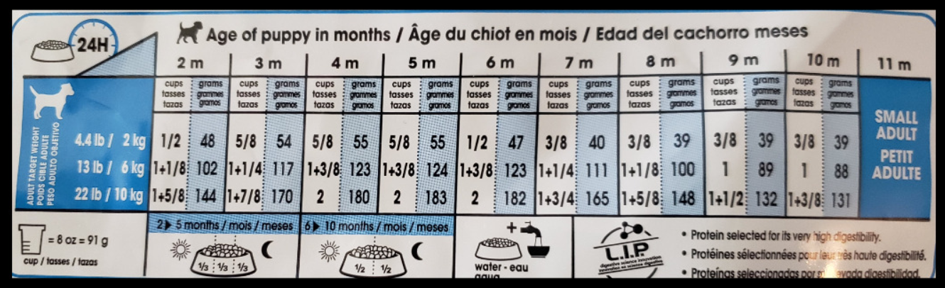
This food chart is basically a conditional statement matrix where you match the conditions on the left side with those on the top to figure out how much to feed your dog.16
So if we wanted to figure out how much to feed a dog that is three months old and will be 4.4 pounds, we’d use the first row on the left (which says 4.4 pounds/2.2 kilograms) and the second column (which says three months old). When the dog gets to be four-months-old we’d keep the same row but now move one column to the right. In normal English you’d say that the dog is four months old and their expected size is 4.4 pounds (2 kg). The language when talking about (and writing code for) a conditional statement in programming is a bit more formal where every condition is spoken as a yes or no question. Here we ask is the dog four months old and is the expected weight 4.4 pounds? If both are true, then we give the dog the amount of food shown for those conditions. If only one is true, then the whole thing is wrong - we wouldn’t want to underfeed or overfeed our dog. In this example, a four month old dog can eat between 5/8th of a cup of food and 2 cups depending on their expected size. So having only one condition be true isn’t enough.
Can you see any issue with this conditional statement matrix? It doesn’t cover the all possible choices for age and weight combinations. In fact, it is really quite narrow in what it does cover. For example, it covers two- and three-months, but not any age in between. We can assume that a dog that is 2.5 months old would eat the average of two and three month meal amounts, but wouldn’t know for sure. When making your own statements please consider what conditions you are checking for - and, importantly, what you’re leaving out.
For a real data example, let’s say you have crime data from every state between 1960 and 2020. Your research question is “did Colorado’s marijuana legalization affect crime in the state?” In that case you want only data from Colorado. Since legalization began in January 2014, you wouldn’t need every year, only years some period of time before and after legalization to be able to measure its effect. So you would need to subset based on the state and the year.
To make conditional statements with multiple conditions we use | for “or” and & for “and”.
Condition 1 | Condition 2
2 == 3 | 2 > 1
# [1] TRUE
As it sounds, when using | as long as at least one condition is true (we can include as many conditions as we like) it will return TRUE.
Condition 1 & Condition 2
2 == 3 & 2 > 1
# [1] FALSE
For &, all of the conditions must be true. If even one condition is not true it will return FALSE.
10.3 Subsetting a data.frame
Earlier we were using a simple vector. In this book - and in your own work - you will usually work on an entire data set. These generally come in the form called a “data.frame,” which you can imagine as being like an Excel file with multiple rows and columns. Section 3.3.2 covers data.frames in more detail.
Let’s load in data from the Uniform Crime Report (UCR), an FBI data set that we’ll work on in a later lesson. This data has crime data every year from 1960-2020 and for nearly every agency in the country.
ucr <- readRDS("data/offenses_known_yearly_1960_2020.rds")Let’s peek at the first 6 rows and 6 columns using the square bracket notation [] for data.frames, which we’ll explain more below.
ucr[1:6, 1:6]
#       ori      ori9 agency_name  state state_abb year
# 1 AK00101 AK0010100   anchorage alaska        AK 2020
# 2 AK00101 AK0010100   anchorage alaska        AK 2019
# 3 AK00101 AK0010100   anchorage alaska        AK 2018
# 4 AK00101 AK0010100   anchorage alaska        AK 2017
# 5 AK00101 AK0010100   anchorage alaska        AK 2016
# 6 AK00101 AK0010100   anchorage alaska        AK 2015
The first 6 rows appear to be agency identification info for Anchorage, Alaska, from 2015-2020. For good measure let’s check how many rows and columns are in this data. This will give us some guidance on subsetting, which we’ll see below. nrow() gives us the number of rows and ncol() gives us the number of columns.
nrow(ucr)
# [1] 1032307ncol(ucr)
# [1] 222This is a large file with 223 columns and over a million rows. Normally we wouldn’t want to print out the names of all 223 columns, but let’s do so here as we want to know the variables available to subset. We can use names() to see the name of every column in a data.frame. Inside the parentheses we put the data.frame name (without quotes).
names(ucr)
#   [1] "ori"                              "ori9"
#   [3] "agency_name"                      "state"
#   [5] "state_abb"                        "year"
#   [7] "number_of_months_missing"         "last_month_reported"
#   [9] "arson_number_of_months_missing"   "arson_last_month_reported"
#  [11] "fips_state_code"                  "fips_county_code"
#  [13] "fips_state_county_code"           "fips_place_code"
#  [15] "agency_type"                      "crosswalk_agency_name"
#  [17] "census_name"                      "longitude"
#  [19] "latitude"                         "address_name"
#  [21] "address_street_line_1"            "address_street_line_2"
#  [23] "address_city"                     "address_state"
#  [25] "address_zip_code"                 "population_group"
#  [27] "population_1"                     "population_1_county"
#  [29] "population_2"                     "population_2_county"
#  [31] "population_3"                     "population_3_county"
#  [33] "population"                       "country_division"
#  [35] "juvenile_age"                     "core_city_indication"
#  [37] "fbi_field_office"                 "followup_indication"
#  [39] "zip_code"                         "month_included_in"
#  [41] "covered_by_ori"                   "agency_count"
#  [43] "special_mailing_address"          "first_line_of_mailing_address"
#  [45] "second_line_of_mailing_address"   "third_line_of_mailing_address"
#  [47] "fourth_line_of_mailing_address"   "officers_killed_by_felony"
#  [49] "officers_killed_by_accident"      "officers_assaulted"
#  [51] "actual_murder"                    "actual_manslaughter"
#  [53] "actual_rape_total"                "actual_rape_by_force"
#  [55] "actual_rape_attempted"            "actual_robbery_total"
#  [57] "actual_robbery_with_a_gun"        "actual_robbery_with_a_knife"
#  [59] "actual_robbery_other_weapon"      "actual_robbery_unarmed"
#  [61] "actual_assault_total"             "actual_assault_with_a_gun"
#  [63] "actual_assault_with_a_knife"      "actual_assault_other_weapon"
#  [65] "actual_assault_unarmed"           "actual_assault_simple"
#  [67] "actual_burg_total"                "actual_burg_force_entry"
#  [69] "actual_burg_nonforce_entry"       "actual_burg_attempted"
#  [71] "actual_theft_total"               "actual_mtr_veh_theft_total"
#  [73] "actual_mtr_veh_theft_car"         "actual_mtr_veh_theft_truck"
#  [75] "actual_mtr_veh_theft_other"       "actual_all_crimes"
#  [77] "actual_assault_aggravated"        "actual_index_violent"
#  [79] "actual_index_property"            "actual_index_total"
#  [81] "actual_arson_single_occupancy"    "actual_arson_other_residential"
#  [83] "actual_arson_storage"             "actual_arson_industrial"
#  [85] "actual_arson_other_commercial"    "actual_arson_community_public"
#  [87] "actual_arson_all_oth_structures"  "actual_arson_total_structures"
#  [89] "actual_arson_motor_vehicles"      "actual_arson_other_mobile"
#  [91] "actual_arson_total_mobile"        "actual_arson_all_other"
#  [93] "actual_arson_grand_total"         "tot_clr_murder"
#  [95] "tot_clr_manslaughter"             "tot_clr_rape_total"
#  [97] "tot_clr_rape_by_force"            "tot_clr_rape_attempted"
#  [99] "tot_clr_robbery_total"            "tot_clr_robbery_with_a_gun"
# [101] "tot_clr_robbery_with_a_knife"     "tot_clr_robbery_other_weapon"
# [103] "tot_clr_robbery_unarmed"          "tot_clr_assault_total"
# [105] "tot_clr_assault_with_a_gun"       "tot_clr_assault_with_a_knife"
# [107] "tot_clr_assault_other_weapon"     "tot_clr_assault_unarmed"
# [109] "tot_clr_assault_simple"           "tot_clr_burg_total"
# [111] "tot_clr_burg_force_entry"         "tot_clr_burg_nonforce_entry"
# [113] "tot_clr_burg_attempted"           "tot_clr_theft_total"
# [115] "tot_clr_mtr_veh_theft_total"      "tot_clr_mtr_veh_theft_car"
# [117] "tot_clr_mtr_veh_theft_truck"      "tot_clr_mtr_veh_theft_other"
# [119] "tot_clr_all_crimes"               "tot_clr_assault_aggravated"
# [121] "tot_clr_index_violent"            "tot_clr_index_property"
# [123] "tot_clr_index_total"              "tot_clr_arson_single_occupancy"
# [125] "tot_clr_arson_other_residential"  "tot_clr_arson_storage"
# [127] "tot_clr_arson_industrial"         "tot_clr_arson_other_commercial"
# [129] "tot_clr_arson_community_public"   "tot_clr_arson_all_oth_structures"
# [131] "tot_clr_arson_total_structures"   "tot_clr_arson_motor_vehicles"
# [133] "tot_clr_arson_other_mobile"       "tot_clr_arson_total_mobile"
# [135] "tot_clr_arson_all_other"          "tot_clr_arson_grand_total"
# [137] "clr_18_murder"                    "clr_18_manslaughter"
# [139] "clr_18_rape_total"                "clr_18_rape_by_force"
# [141] "clr_18_rape_attempted"            "clr_18_robbery_total"
# [143] "clr_18_robbery_with_a_gun"        "clr_18_robbery_with_a_knife"
# [145] "clr_18_robbery_other_weapon"      "clr_18_robbery_unarmed"
# [147] "clr_18_assault_total"             "clr_18_assault_with_a_gun"
# [149] "clr_18_assault_with_a_knife"      "clr_18_assault_other_weapon"
# [151] "clr_18_assault_unarmed"           "clr_18_assault_simple"
# [153] "clr_18_burg_total"                "clr_18_burg_force_entry"
# [155] "clr_18_burg_nonforce_entry"       "clr_18_burg_attempted"
# [157] "clr_18_theft_total"               "clr_18_mtr_veh_theft_total"
# [159] "clr_18_mtr_veh_theft_car"         "clr_18_mtr_veh_theft_truck"
# [161] "clr_18_mtr_veh_theft_other"       "clr_18_all_crimes"
# [163] "clr_18_assault_aggravated"        "clr_18_index_violent"
# [165] "clr_18_index_property"            "clr_18_index_total"
# [167] "clr_18_arson_single_occupancy"    "clr_18_arson_other_residential"
# [169] "clr_18_arson_storage"             "clr_18_arson_industrial"
# [171] "clr_18_arson_other_commercial"    "clr_18_arson_community_public"
# [173] "clr_18_arson_all_oth_structures"  "clr_18_arson_total_structures"
# [175] "clr_18_arson_motor_vehicles"      "clr_18_arson_other_mobile"
# [177] "clr_18_arson_total_mobile"        "clr_18_arson_all_other"
# [179] "clr_18_arson_grand_total"         "unfound_murder"
# [181] "unfound_manslaughter"             "unfound_rape_total"
# [183] "unfound_rape_by_force"            "unfound_rape_attempted"
# [185] "unfound_robbery_total"            "unfound_robbery_with_a_gun"
# [187] "unfound_robbery_with_a_knife"     "unfound_robbery_other_weapon"
# [189] "unfound_robbery_unarmed"          "unfound_assault_total"
# [191] "unfound_assault_with_a_gun"       "unfound_assault_with_a_knife"
# [193] "unfound_assault_other_weapon"     "unfound_assault_unarmed"
# [195] "unfound_assault_simple"           "unfound_burg_total"
# [197] "unfound_burg_force_entry"         "unfound_burg_nonforce_entry"
# [199] "unfound_burg_attempted"           "unfound_theft_total"
# [201] "unfound_mtr_veh_theft_total"      "unfound_mtr_veh_theft_car"
# [203] "unfound_mtr_veh_theft_truck"      "unfound_mtr_veh_theft_other"
# [205] "unfound_all_crimes"               "unfound_assault_aggravated"
# [207] "unfound_index_violent"            "unfound_index_property"
# [209] "unfound_index_total"              "unfound_arson_single_occupancy"
# [211] "unfound_arson_other_residential"  "unfound_arson_storage"
# [213] "unfound_arson_industrial"         "unfound_arson_other_commercial"
# [215] "unfound_arson_community_public"   "unfound_arson_all_oth_structures"
# [217] "unfound_arson_total_structures"   "unfound_arson_motor_vehicles"
# [219] "unfound_arson_other_mobile"       "unfound_arson_total_mobile"
# [221] "unfound_arson_all_other"          "unfound_arson_grand_total"
Now let’s discuss how to subset this data into a smaller data set to answer a specific question. Let’s subset the data to answer our above question of “did Colorado’s marijuana legalization affect crime in the state?” Like mentioned above, we need data just from Colorado and just for years around the legalization year - we can do 2011-2017 for simplicity.
We also don’t need all 223 columns in the current data. Let’s say we’re only interested in whether murder changes. We’d need the column called actual_murder, the state column (as a check to make sure we subset only Colorado), the year column, the population column, the ori column, and the agency_name column (a real analysis would likely grab geographic variables too to see if changes depended on location, but here we’re just using it as an example). The last two columns - ori and agency_name - aren’t strictly necessary but would be useful for checking if an agency’s values are reasonable (e.g. see if that agency had a sudden huge spike or decline in reported crimes) when checking for outliers, a step we won’t do here.
Before explaining how to subset from a data.frame, let’s write pseudocode (essentially a description of what we are going to do that is readable to people but isn’t real code) for our subset.
We want
- Only rows where the state equals Colorado
- Only rows where the year is 2011-2017
- Only the following columns: actual_murder, state, year, population, ori, agency_name
10.3.1 Select specific columns
The way to select a specific column in R is called the dollar sign notation.
data$column
We write the data name followed by a $ and then the column name. Make sure there are no spaces, quotation marks, or misspellings (or capitalization issues). Just the data$column exactly as it is spelled. Since we are referring to data already read into R, there should not be any quotes for either the data or the column name.
We can do this for the column agency_name in our UCR data. If we wrote this in the console it would print out every single row in the column. Because this data is large (over a million rows), I am going to wrap this in head() so it only displays the first 6 rows of the column rather than printing the entire column.
head(ucr$agency_name)
# [1] "anchorage" "anchorage" "anchorage" "anchorage" "anchorage" "anchorage"
They’re all the same name because Anchorage Police reported many times and are in the data set multiple times. Let’s look at the column actual_murder, which shows the annual number of murders in that agency.
head(ucr$actual_murder)
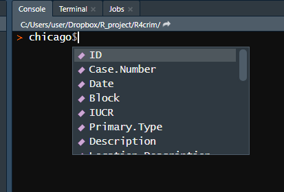
# [1] 18 32 26 27 28 26One hint is to write out the data set name in the console and hit the Tab key. Wait a couple of seconds and a popup will appear listing every column in the data set. You can scroll through this and then hit enter to select that column.
10.3.2 Select specific rows
In the earlier examples, we used square bracket notation [] and just put a number or several numbers in the []. When dealing with data.frames, however, you need an extra step to tell R which columns to keep. The syntax in the square bracket is
[row, column]
We start the square bracket by saying which row we want. Now, since we also have to consider the columns, we need to tell it the number or name (in a vector using c() if more than one name and putting column names in quotes) of the column or columns we want.
The exception to this is when we use the dollar sign notation to select a single column. In that case we don’t need a comma (and indeed it will give us an error!). Let’s see a few examples and then explain why this works the way it does.
ucr[1, 1]
# [1] "AK00101"
If we input multiple numbers, we can get multiple rows and columns.
ucr[1:6, 1:6]
#       ori      ori9 agency_name  state state_abb year
# 1 AK00101 AK0010100   anchorage alaska        AK 2020
# 2 AK00101 AK0010100   anchorage alaska        AK 2019
# 3 AK00101 AK0010100   anchorage alaska        AK 2018
# 4 AK00101 AK0010100   anchorage alaska        AK 2017
# 5 AK00101 AK0010100   anchorage alaska        AK 2016
# 6 AK00101 AK0010100   anchorage alaska        AK 2015
The column section also accepts a vector of the names of the columns. These names must be spelled correctly and in quotes.
ucr[1:6, c("ori", "year")]
#       ori year
# 1 AK00101 2020
# 2 AK00101 2019
# 3 AK00101 2018
# 4 AK00101 2017
# 5 AK00101 2016
# 6 AK00101 2015
In cases where we want every row or every column, we just don’t put a number. By default, R will return every row/column if you don’t specify which ones you want. However, you will still need to include the comma.
Here is every column in the first row. Again, for real work we’d likely not do this as it will print out hundreds of rows to the console.
ucr[1, ]
#       ori      ori9 agency_name  state state_abb year number_of_months_missing
# 1 AK00101 AK0010100   anchorage alaska        AK 2020                        0
#   last_month_reported arson_number_of_months_missing arson_last_month_reported
# 1            december                              0                  december
#   fips_state_code fips_county_code fips_state_county_code fips_place_code
# 1              02              020                  02020           03000
#               agency_type       crosswalk_agency_name            census_name
# 1 local police department anchorage police department anchorage municipality
#     longitude latitude                address_name address_street_line_1
# 1 -149.284329 61.17425 anchorage police department        4501 elmore rd
#   address_street_line_2 address_city address_state address_zip_code
# 1                  <NA>    anchorage            ak            99507
#            population_group population_1 population_1_county population_2
# 1 city 250,000 thru 499,999       286388                   0            0
#   population_2_county population_3 population_3_county population
# 1                  NA            0                  NA     286388
#   country_division juvenile_age core_city_indication fbi_field_office
# 1          pacific           NA     core city of msa             3030
#       followup_indication zip_code month_included_in covered_by_ori
# 1 do not send a follow-up    99507                 0           <NA>
#   agency_count       special_mailing_address first_line_of_mailing_address
# 1            1 not a special mailing address                4501 elmore rd
#   second_line_of_mailing_address third_line_of_mailing_address
# 1                           <NA>                          <NA>
#   fourth_line_of_mailing_address officers_killed_by_felony
# 1                           <NA>                         0
#   officers_killed_by_accident officers_assaulted actual_murder
# 1                           0                464            18
#   actual_manslaughter actual_rape_total actual_rape_by_force
# 1                   0               558                  534
#   actual_rape_attempted actual_robbery_total actual_robbery_with_a_gun
# 1                    24                  558                       124
#   actual_robbery_with_a_knife actual_robbery_other_weapon
# 1                          65                          82
#   actual_robbery_unarmed actual_assault_total actual_assault_with_a_gun
# 1                    287                 5777                       512
#   actual_assault_with_a_knife actual_assault_other_weapon
# 1                         377                         840
#   actual_assault_unarmed actual_assault_simple actual_burg_total
# 1                    609                  3439              1444
#   actual_burg_force_entry actual_burg_nonforce_entry actual_burg_attempted
# 1                     900                        453                    91
#   actual_theft_total actual_mtr_veh_theft_total actual_mtr_veh_theft_car
# 1               7279                       1149                      807
#   actual_mtr_veh_theft_truck actual_mtr_veh_theft_other actual_all_crimes
# 1                        278                         64             16856
#   actual_assault_aggravated actual_index_violent actual_index_property
# 1                      2338                 3472                  9945
#   actual_index_total actual_arson_single_occupancy
# 1              13417                             6
#   actual_arson_other_residential actual_arson_storage actual_arson_industrial
# 1                             16                    1                       0
#   actual_arson_other_commercial actual_arson_community_public
# 1                            10                             7
#   actual_arson_all_oth_structures actual_arson_total_structures
# 1                               0                            30
#   actual_arson_motor_vehicles actual_arson_other_mobile
# 1                          17                         0
#   actual_arson_total_mobile actual_arson_all_other actual_arson_grand_total
# 1                        17                      0                       73
#   tot_clr_murder tot_clr_manslaughter tot_clr_rape_total tot_clr_rape_by_force
# 1             15                    0                 46                    41
#   tot_clr_rape_attempted tot_clr_robbery_total tot_clr_robbery_with_a_gun
# 1                      5                   207                         30
#   tot_clr_robbery_with_a_knife tot_clr_robbery_other_weapon
# 1                           33                           27
#   tot_clr_robbery_unarmed tot_clr_assault_total tot_clr_assault_with_a_gun
# 1                     117                  3407                        223
#   tot_clr_assault_with_a_knife tot_clr_assault_other_weapon
# 1                          281                          511
#   tot_clr_assault_unarmed tot_clr_assault_simple tot_clr_burg_total
# 1                     428                   1964                237
#   tot_clr_burg_force_entry tot_clr_burg_nonforce_entry tot_clr_burg_attempted
# 1                      115                         118                      4
#   tot_clr_theft_total tot_clr_mtr_veh_theft_total tot_clr_mtr_veh_theft_car
# 1                 865                         197                       153
#   tot_clr_mtr_veh_theft_truck tot_clr_mtr_veh_theft_other tot_clr_all_crimes
# 1                          39                           5               5001
#   tot_clr_assault_aggravated tot_clr_index_violent tot_clr_index_property
# 1                       1443                  1711                   1326
#   tot_clr_index_total tot_clr_arson_single_occupancy
# 1                3037                              2
#   tot_clr_arson_other_residential tot_clr_arson_storage
# 1                               8                     0
#   tot_clr_arson_industrial tot_clr_arson_other_commercial
# 1                        0                              5
#   tot_clr_arson_community_public tot_clr_arson_all_oth_structures
# 1                              3                                0
#   tot_clr_arson_total_structures tot_clr_arson_motor_vehicles
# 1                             13                            5
#   tot_clr_arson_other_mobile tot_clr_arson_total_mobile tot_clr_arson_all_other
# 1                          0                          5                       0
#   tot_clr_arson_grand_total clr_18_murder clr_18_manslaughter clr_18_rape_total
# 1                        27             0                   0                11
#   clr_18_rape_by_force clr_18_rape_attempted clr_18_robbery_total
# 1                   11                     0                    5
#   clr_18_robbery_with_a_gun clr_18_robbery_with_a_knife
# 1                         2                           0
#   clr_18_robbery_other_weapon clr_18_robbery_unarmed clr_18_assault_total
# 1                           1                      2                  228
#   clr_18_assault_with_a_gun clr_18_assault_with_a_knife
# 1                        18                          13
#   clr_18_assault_other_weapon clr_18_assault_unarmed clr_18_assault_simple
# 1                          25                     12                   160
#   clr_18_burg_total clr_18_burg_force_entry clr_18_burg_nonforce_entry
# 1                 4                       4                          0
#   clr_18_burg_attempted clr_18_theft_total clr_18_mtr_veh_theft_total
# 1                     0                 36                          9
#   clr_18_mtr_veh_theft_car clr_18_mtr_veh_theft_truck
# 1                        8                          1
#   clr_18_mtr_veh_theft_other clr_18_all_crimes clr_18_assault_aggravated
# 1                          0               295                        68
#   clr_18_index_violent clr_18_index_property clr_18_index_total
# 1                   84                    51                135
#   clr_18_arson_single_occupancy clr_18_arson_other_residential
# 1                             0                              0
#   clr_18_arson_storage clr_18_arson_industrial clr_18_arson_other_commercial
# 1                    0                       0                             0
#   clr_18_arson_community_public clr_18_arson_all_oth_structures
# 1                             0                               0
#   clr_18_arson_total_structures clr_18_arson_motor_vehicles
# 1                             0                           0
#   clr_18_arson_other_mobile clr_18_arson_total_mobile clr_18_arson_all_other
# 1                         0                         0                      0
#   clr_18_arson_grand_total unfound_murder unfound_manslaughter
# 1                        2              4                    0
#   unfound_rape_total unfound_rape_by_force unfound_rape_attempted
# 1                  1                     1                      0
#   unfound_robbery_total unfound_robbery_with_a_gun unfound_robbery_with_a_knife
# 1                     0                          0                            0
#   unfound_robbery_other_weapon unfound_robbery_unarmed unfound_assault_total
# 1                            0                       0                     0
#   unfound_assault_with_a_gun unfound_assault_with_a_knife
# 1                          0                            0
#   unfound_assault_other_weapon unfound_assault_unarmed unfound_assault_simple
# 1                            0                       0                      0
#   unfound_burg_total unfound_burg_force_entry unfound_burg_nonforce_entry
# 1                  4                        2                           1
#   unfound_burg_attempted unfound_theft_total unfound_mtr_veh_theft_total
# 1                      1                  43                          37
#   unfound_mtr_veh_theft_car unfound_mtr_veh_theft_truck
# 1                        22                          15
#   unfound_mtr_veh_theft_other unfound_all_crimes unfound_assault_aggravated
# 1                           0                 89                          0
#   unfound_index_violent unfound_index_property unfound_index_total
# 1                     5                     84                  89
#   unfound_arson_single_occupancy unfound_arson_other_residential
# 1                              0                               0
#   unfound_arson_storage unfound_arson_industrial unfound_arson_other_commercial
# 1                     0                        0                              0
#   unfound_arson_community_public unfound_arson_all_oth_structures
# 1                              0                                0
#   unfound_arson_total_structures unfound_arson_motor_vehicles
# 1                              0                            0
#   unfound_arson_other_mobile unfound_arson_total_mobile unfound_arson_all_other
# 1                          0                          0                       0
#   unfound_arson_grand_total
# 1                         0
Since there are 223 columns in our data, normally we’d want to avoid printing out all of them. And in most cases, we would save the output of subsets to a new object to be used later rather than just printing the output in the console.
What happens if we forget the comma? If we put in numbers for both rows and columns but don’t include a comma between them it will have an error.
ucr[1 1]
# Error: <text>:1:7: unexpected numeric constant
# 1: ucr[1 1
#           ^
If we only put in a single number and no comma, it will return the column that matches that number. Here we have number 1 and it will return the first column. We’ll wrap it in head() so it doesn’t print out a million rows.
head(ucr[1])
#       ori
# 1 AK00101
# 2 AK00101
# 3 AK00101
# 4 AK00101
# 5 AK00101
# 6 AK00101
Since R thinks you are requesting a column, and we only have 223 columns in the data, asking for any number above 223 will return an error.
head(ucr[1000])
# Error in `[.data.frame`(ucr, 1000): undefined columns selected
If you already specify a column using dollar sign notation $, you do not need to indicate any column in the square brackets[]. All you need to do is say which row or rows you want.
ucr$agency_name[15]
# [1] "anchorage"
10.3.3 Subset Colorado data
Now we have the tools to subset our UCR data to just be Colorado from 2011-2017. There are three conditional statements we need to make, two for rows and one for columns.
- Only rows where the state equals Colorado
- Only rows where the year is 2011-2017
- Only the following columns: actual_murder, state, year, population, ori, agency_name
We could use the & operator to say rows must meet condition 1 and condition 2. Since this is an intro lesson, we will do them as two separate conditional statements. For the first step we want to get all rows in the data where the state equals “colorado” (in this data all state names are lowercase). And at this point we want to keep all columns in the data. So let’s make a new object called colorado to save the result of this subset.
Remember that we want to put the object to the left of the [] (and touching the []) to make sure it returns the data. Just having the conditional statement will only return TRUE or FALSE values. Since we want all columns, we don’t need to put anything after the comma (but we must include the comma!).
colorado <- ucr[ucr$state == "colorado", ]Now we want to get all the rows where the year is 2011-2017. Since we want to check if the year is one of the years 2011-2017, we will use %in% and put the years in a vector 2011:2017. This time our primary data set is colorado, not ucr since colorado has already subsetted to just the state we want. This is how subsetting generally works. You take a large data set, subset it to a smaller one and continue to subset the smaller one to only the data you want.
colorado <- colorado[colorado$year %in% 2011:2017, ]Finally we want the columns stated above and to keep every row in the current data. Since the format is [row, column] in this case we keep the “row” part blank to indicate that we want every row.
colorado <- colorado[ , c("actual_murder",
                          "state",
                          "year",
                          "population",
                          "ori",
                          "agency_name")]
We can do a quick check using the unique() function. The unique() function prints all the unique values in a category, such as a column. We will use it on the state and year columns to make sure only the values that we want are present.
unique(colorado$state)
# [1] "colorado"unique(colorado$year)
# [1] 2017 2016 2015 2014 2013 2012 2011The only state is Colorado and the only years are 2011-2017 so our subset worked! This data shows the number of murders in each agency. We want to look at state trends so in Section 11.3 we will sum up all the murders per year and see if marijuana legalization affected it.
10.3.3.1 Subsetting using dplyr
Above, we did subsetting through what’s called the “base R” method. “Base R” just means that we use functions that are built into R and don’t use any packages. A very popular alternative way to do most of the work done in this chapter is to use the dplyr package. dplyr is a very useful package to handle data and includes functions that let us subset data, select only certain columns, and aggregate the data. For the package’s website, which covers all of the features in this package, please see here.
dplyr is part of what is called the “tidyverse,” which is a collection of R packages written by mostly the same people that include lots of functions that are useful for working with the kind of data we use in this book. We’ll cover many of the tidyverse packages in this book. There’s nothing special about a package being a “tidyverse” package; they operate exactly the same as other packages. I just mention it because it is a very popular set of packages, and people will often talk about “tidyverse” approaches to R meaning using these packages. So it’s good to know the terminology. To look at the full list of tidyverse packages, their website here is an excellent overview of them.
In a lot of ways the functions we’ll use from dplyr are simpler and easier to use than what we wrote earlier in this chapter. In fact, a lot of people learn only dplyr functions and do not learn (or at least do not spend much time on) base R. For the rest of this book we’ll use base R and tidyverse functions alongside each other. I do this for two reasons. First, it’s important to understand how R works and using base R is the best way to learn. This is a programming-for-a-purpose book, not a pure programming book, so the focus isn’t on knowing all the ins and outs of R. However, I think it is still important to have some understanding of how R works and tidyverse functions tend to obfuscate that.
In most cases this obfuscation is a good thing as it lets you focus on working with the data instead of thinking about how R works (and this is one of the tidyverse authors’ motivations behind their work). In some cases, however, you’ll encounter issues with either the code or your data where its important to understand how R works. In these (luckily relatively) rare cases, base R tends to be more useful in solving these problems than the tidyverse.
The second reason is that base R functions are incredibly stable. Most haven’t changed since R was first created in the early 1990s. The benefit is that code you write using base R functions will work for a very long time. Using packages outside of base R (all packages, not just tidyverse packages) always carries the risk that a new version of the package will change the behavior of a function, or remove that function entirely. Thankfully this is quite rare as package developers often take care to ensure that old features remain available even as they update their package. But it is always a risk, and for programming for research we want to try to make our code as reproducible as possible, which means trying to ensure that functions we use will keep working in the future. That said, please don’t avoid packages too much out of fear of this issue. Packages in R are enormously useful, and we’ll use many of them throughout this book.
We’ll cover two functions from dplyr here, and we’ll also cover a couple more in the next chapter. For now, we’ll look only at filter() and select(). The filter() function is how dplyr does subsetting. It takes a conditional statement and “filters” the data to only return rows where that conditional statement is true. You can include multiple conditional statements in the parentheses of filter() and it’ll return only rows where all of the statements are true. The select() function does roughly that with columns where we can input a conditional statement about the name of the column (e.g. columns ending in “rate”) and it’ll return only those columns. select() also lets you choose columns just by putting the name of the column(s) in the parentheses and that’s all we’ll be using it for here.
Let’s first copy back some of the code we used earlier when we used base R to subset Colorado data from the UCR data set.
colorado <- ucr[ucr$state == "colorado", ]
colorado <- colorado[colorado$year %in% 2011:2017, ]
colorado <- colorado[ , c("actual_murder",
                          "state",
                          "year",
                          "population",
                          "ori",
                          "agency_name")]
We have two conditional statements - keep only rows where state is Colorado and where years are between 2011 and 2017 (including 2017) - and then we kept only a small number of columns.
We’ll do this one step at a time using the dplyr functions. For filter() we first include the name of our data.frame, which in this case starts as “ucr” and then becomes “colorado” as we make a new object during the first line of code, and then we include our conditional statement. Using base R, we have to say which data.frame we used every time we included a column. Using filter() we don’t need to do this. filter() is smart enough to select the column from the data.frame we input.
For our first filter we can write filter(ucr, state == "colorado") and we will save the resulting object into a data set called “colorado” like we did above. To use any dplyr functions we first need to install that package and then tell R we want to use it through the library() function.
install.packages("dplyr")library(dplyr)
#
# Attaching package: 'dplyr'
# The following objects are masked from 'package:stats':
#
# filter, lag
# The following objects are masked from 'package:base':
#
# intersect, setdiff, setequal, union
colorado <- filter(ucr, state == "colorado")Now we can do our second conditional statement where we keep only years 2011 through 2017.
colorado <- filter(ucr, year %in% 2011:2017)If we wanted to, we could combine these lines of code into a single line by including both conditional statements into a single filter() function by just including a comma after the first statement.
colorado <- filter(ucr, state == "colorado", year %in% 2011:2017)We follow similar syntax for select() by starting with the name of the data set and then the name of every column you want to keep. Unlike in base R we don’t need to put the columns in a vector or to put the names in quotes (though you can put the names in quotes if you’d like). The order you put the column names in is also the order it will arrange them, so this function can be used to reorder your columns.
colorado <- select(colorado, actual_murder, state,
                   year, population, ori, agency_name)
If we run the same checks on unique states and years as we did after our base R code, we’ll get the same results. This shows that our dplyr code did the same thing as our base R code.
unique(colorado$state)
# [1] "colorado"unique(colorado$year)
# [1] 2017 2016 2015 2014 2013 2012 2011Some languages use “zero indexing,” which means the first index is index 0, the second is index 1. So in our example “cat” would be index 0. R does not do that, and the first value is index 1, the second is index 2, and so on.↩︎
If you encounter some conditional statements that confuse you - which will be more common as you combine many statements together - I encourage you to make a matrix like this yourself. Even if it isn’t that complicated, I think it’s easier to see it written down than to try to keep all of the possible conditions in your head.↩︎