2 Introduction to R and RStudio
In this chapter you’ll learn to open a data file in R. That file is “ucr2017.rda,” which you’ll need to download from the data repository available here.
2.1 Using RStudio
In this lesson we’ll start by looking at RStudio then write some brief code to load in some crime data and start exploring it. This lesson will cover code that you won’t understand completely yet. That is fine, we’ll cover everything in more detail as the lessons progress.
RStudio is the interface we use to work with R. It has a number of features to make it easier for us to work with R. While not strictly necessary to use, most people who use R do so through RStudio. When using R you don’t need to open up both R and RStudio on your computer. Just open RStudio and it’ll internally use R. We’ll spend some time right now looking at RStudio and the options you can change to make it easier to use (and to suit your personal preferences with appearance) as this will make all of the work that we do in this book easier.
When you open up RStudio you’ll see four panels, each of which plays an important role in RStudio. Your RStudio may not look like the setup I have in the following image - that is fine, we’ll learn how to change the appearance of RStudio soon.
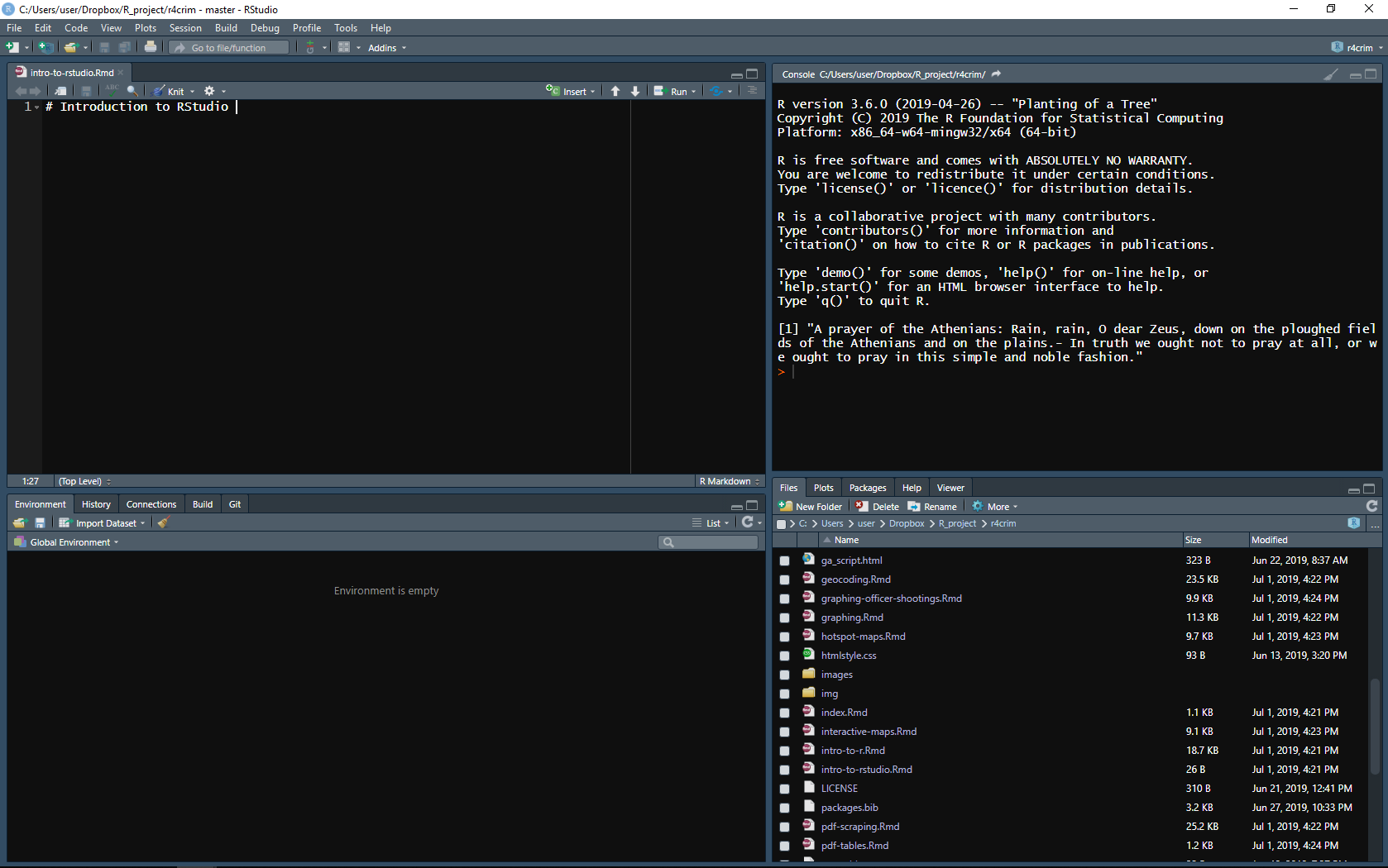
At the top right of the image (and this may be in a different location on your RStudio) is the Console panel. Here you can write code, hit enter/return, and R will run that code. If you write 2+2 it will return (in this case that just mean it will print an answer) 4. This is useful for doing something simple like using R as a calculator or quickly looking at data. In most cases during research this is where you’d do something that you don’t care to keep. This is because when you restart R it won’t save anything written in the Console. To do reproducible research or to be able to collaborate with others you need a way to keep the code you’ve written.
The way to keep the code you’ve written in a file that you can open later or share with someone else is by writing code in an R Script (if you’re familiar with Stata, an R Script is just like a .do file). An R Script is essentially a text file (similar to a Word document) where you write code. To run code in an R Script just click on a line of code or highlight several lines and hit enter/return or click the “Run” button on the top right of the Source panel shown in the top left of the above image. You’ll see the lines of code run in the Console and any output (if your code has an output) will be shown there too (making a plot will be shown in a different panel as we’ll see soon).
For code that you don’t want to run, called comments, start the line with a pound sign # and that line will not be run (it will still print in the console if you run it but it won’t do anything). These comments should explain the code you wrote (if it’s not otherwise obvious what the code does).
It is good practice to do all of your code writing in an R Script - even if you delete some lines of code later - as it eliminates the possibility of losing code or forgetting what you wrote. Having all the code in front of you in a text file also makes it easier to understand the flow of code from start to finish for a task - an issue we’ll discuss more in later lessons.
While the Source and Console panels are the ones that are of most use, there are two other panels worth discussing. As these two panels let you interchange which tabs are available in them, we’ll return to them shortly in the discussion of the options RStudio has to customize it.
2.1.1 Opening an R Script
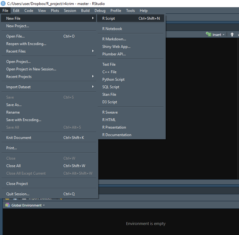
When you want to open up a new R Script you can click File on the very top left, then R Script. It will open up the script in a new tab inside of the Source panel. There are also a number of other file options available: R Presentation which can make PowerPoints; R Markdown, which can make Word Documents or PDFs that incorporate R code used to make tables or graphs (and which we’ll cover in Chapter 7); and Shiny Web App to make websites using R. There is too much to cover for an introductory book such as this, but keep in mind the wide capabilities of R if you have another task to do. To open an R Script that is already saved to your computer, click “Open File…” and navigate to the file that you want to open.
2.1.2 Setting the working directory
Many research projects incorporate data that someone else (such as the FBI or a local police agency) has put together. In these cases, we need to load the data into R to be able to use it. In a little bit we’ll load a data set into R and start working on it, but let’s take a step back now and think about how to even load data. First, we’ll need to get the data onto our computer somehow, probably by downloading it from an agency’s website. Let’s be specific - we don’t download it to our computer, we download it to a specific folder on our computer (usually defaulted to the Downloads folder on a Windows machine). So let’s say you wanted to load a file called “data” into R. If you have a file called “data” in both your Desktop and your Downloads folder, R wouldn’t know which one you wanted. And unless your data was in the folder R searches by default (which may not be where the file is downloaded by default), R won’t know which file to load.
We need to tell R explicitly which folder has the data to load. We do this by setting the “Working Directory” (or the “Folders where I want you, R, to look for my data” in more simple terms). To set a working directory in R click the Session tab on the top menu, scroll to Set Working Directory, then click Choose Directory. This will open a window where you can navigate to the folder you want.
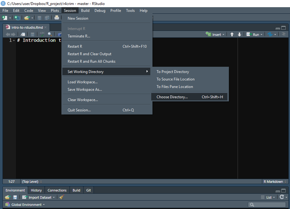
After clicking Open in that window you’ll see a new line of code in the Console starting with setwd() and inside of the parentheses is the route your computer takes to get to the folder you selected. And now R knows which folder to look in for the data you want. It is good form to start your R Script with setwd() to make sure you can load the data. Copy the line of code that says setwd() (which stands for “set working directory”), including everything in the parentheses, to your R Script when you start working.
2.1.3 Changing RStudio
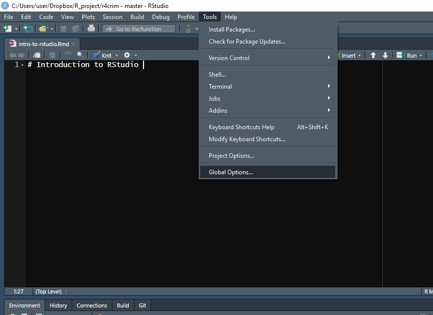
Your RStudio looks different than my RStudio because I changed a number of settings to suit my preferences. To do so yourself click the Tools tab on the top menu and then click Global Options.
This opens up a window with a number of different tabs to change how R behaves and how it looks.
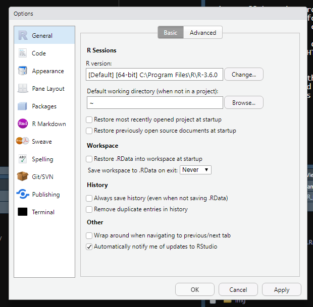
2.1.3.1 General
Under Workspace in the General tab make sure to uncheck the “Restore .RData into workspace at startup” and to set “Save workspace to .RData on exit:” to Never. What this does is make sure that every time you open RStudio it starts fresh with no objects (essentially data loaded into R or made in R) from previous sessions. This may be annoying at times, especially when it comes to loading large files, but the benefits far outweigh the costs.
You want your code to run from start to finish without any errors. Something I’ve seen many students do is write some code in the Console (or in their R Script but out of order of how it should be run) to fix an issue with the data. This means their data is how it should be, but when the R session restarts (such as if the computer restarts) they won’t be able to get back to that point. Making sure your code handles everything from start to finish is well-worth the avoided headache of trying to remember what code you did to fix the issue previously.
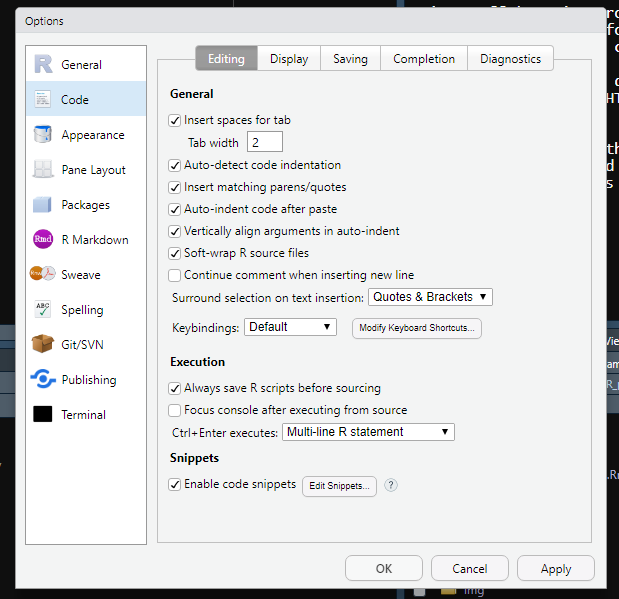
2.1.3.2 Code
The Code tab lets you specify how you want the code to be displayed. The important section for us is to make sure to check the “Soft-wrap R source files” check-box. If you write a very long line of code it gets too big to view all at once and you must scroll to the right to read it all. That can be annoying as you won’t be able to see all the code at once. Setting “Soft-wrap” makes it so if a line is too long it will just be shown on multiple lines, which solves that issue. In practice it is best to avoid long lines of codes as it makes it hard to read, but that isn’t always possible.
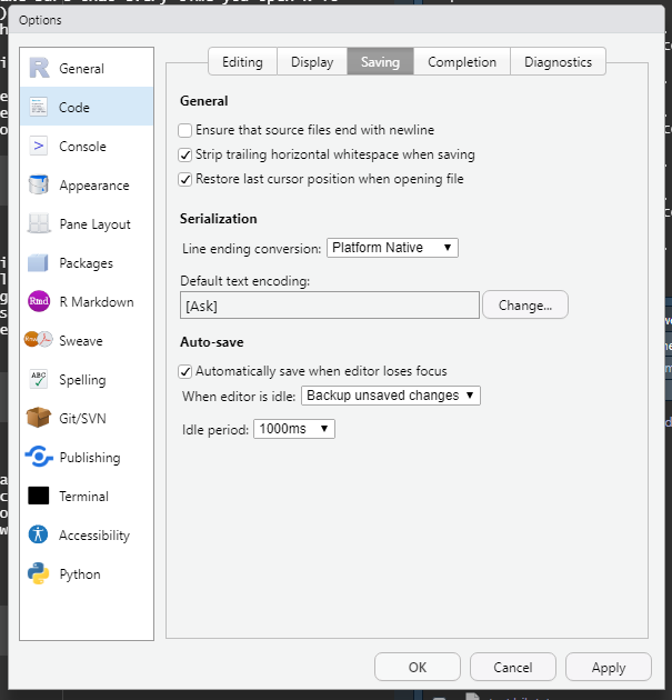
2.1.3.2.1 Saving
Inside of the Code tab we also want to turn on an option to have RStudio automatically save the R script when we aren’t using it. This is like how Google Docs automatically saves your document every second or so. While we should be saving our file often (using the little floppy disk icon near the top of RStudio), having RStudio automatically save adds a level of security as it prevents losing a lot of progress if we forget to save and RStudio crashes or we close it.
To set it to autosave, move to the Saving tab, and check the “Automatically save when editor loses focus” box. So if you click out of RStudio or stop typing, it will automatically save. You can also say how long to wait before saving with options ranging from 500 milliseconds to 10,000 milliseconds, which is the same as 0.5 seconds to 10 seconds.
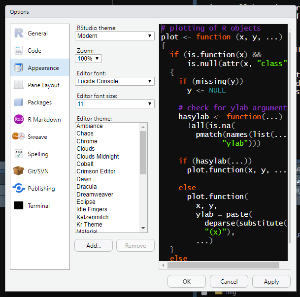
2.1.3.3 Appearance
The Appearance tab lets you change the background, color, and size of text. Change it to your preferences.
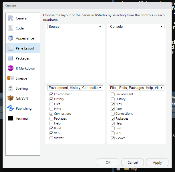
2.1.3.4 Pane Layout
The final tab we’ll look at is Pane Layout. This lets you move around the Source, Console, and the other two panels. There are a number of different tabs to select for the panels (unchecking one just moves it to the other panel, it doesn’t remove it from RStudio), and we’ll talk about three of them. The Environment tab shows every object you load into R or make in R. So if you load a file called “data” you can check the Environment tab. If it is there, you have loaded the file correctly.
As we’ll discuss more in Section 2.3, the Help tab will open up to show you a help page for a function you want more information on (we’ll also discuss exactly what a function is below. But for now just think of a function as a shortcut to using code that someone else wrote). The Plots tab will display any plot you make. It also keeps all plots you’ve made (until restarting RStudio) so you can scroll through the plots.
2.2 Assigning variables
When we’re using R for research the general process is to load data, change it somehow (such as deleting rows we don’t want, aggregating from some small unit such as monthly crime to a higher unit such as yearly crime), and then analyze it. To do all this we need to be able to make sure each step we do actually changes the data. This seems simple but is actually a very common issue I’ve noticed when working with new R programmers - they run code on the data (e.g. deleting certain rows) but forget to save the change to that data.
Let’s look at an example of this. First, we need to know how to create objects in R. I use “object” in a very vague sense to mean anything that is loaded into R and can be manipulated. To create something in R we assign “something” to an object name. This is a very technical sentence so let’s look at an example and then step back and try to understand that sentence.
a <- 1Above I am creating the object “a” by assigning it the value of 1. In R terms, “a is assigned 1” or “a gets 1”. In non-technical terms: a equals 1.
We can print out a to see if this is true.
a
# [1] 1
When we print out a, it returns 1 since that was what a was assigned to. We can assign a another value, and it will overwrite 1 with whatever value we choose.
a <- 33
a
# [1] 33
Now a is 33. Or a equals 33. Or a was assigned 33. Or a gets 33. Or we assigned 33 to a. There are a lot of ways to explain what we did here, which is quite frustrating and confusing to new R programmers. I use the terms “assignment” and “gets” only because that is the convention in R, but if it’s easier for you to talk about something equaling something else (instead of being assigned to that value), please do so!
The <- is what does the assignment, or what makes the thing on the left equal to the thing on the right. You might be thinking that it’d be easier to simply use the equal sign instead of the <- - we are making things equal after all. And you’d be right. Using = does the exact same thing as <-.
a = 13
a
# [1] 13
We can use = instead of <- and get the same results (with very few exceptions and none that are relevant in this book). The reason that people use <- instead of = is largely a matter of convention. It’s just the thing that R programmers do so new programmers tend to adopt it. If it’s easier for you to use = instead of <-, feel free to do that.
In this book I’ll use <- and talk about “assigning” values because that is the convention in R. And while that’s not really a good reason to do anything, I think that it’s important that new R programmers at least know what the proper conventions are and be able to speak the language (so to speak) of R programmers. This is also important when searching for more help on a topic as you need to know the right term to be able to ask for help (from other R programmers and from Google) easily.
So far we’ve just been assigning “a” a value, or overwriting that value with a new value. We can also assign something new to have the same value as a. Let’s make the object “example_123_value.demonstration” get the value that a has - or in other words make “example_123_value.demonstration” be equal to a.
example_123_value.demonstration <- a
example_123_value.demonstration
# [1] 13
I use name “example_123_value.demonstration” just an example of what you can include in an object name - any character (lower or uppercase), any number (just can’t start with a number), and some punctuation (e.g. underscores and periods). Spaces are not allowed. In practice you’ll want to call each object something specific so you know what it is, and ideally make the name as short as possible. For example, if you are using crime data from Houston you’ll want to call it something like “houston_crime”. The R convention is to only use lowercase characters and include only underscores as the punctuation, but you can name it whatever is most useful to you.
As noted at the start of the section, a lot of new programmers will make a change to an object but forget to assign the result back into the object (or into a new object). This means that that object won’t actually change. For example, let’s say we want to multiply example_123_value.demonstration by 10.
If we do example_123_value.demonstration * 10 then it’ll print out the result in the console, but not actually change example_123_value.demonstration. What we need to do is assign that result of the multiplication back into example_123_value.demonstration. Lots of new programmers forget to assign the results back into the object, which understandably leads to lots of confusion since the object is now not what they expect it to be.
example_123_value.demonstration <- example_123_value.demonstration * 10
example_123_value.demonstration
# [1] 130
I’ve been saying “object” a lot, without defining it. An object is a bit tricky to define, especially at this stage in the book. Throughout this book I’ll be using object to describe something that has been assigned value, such as “a” and “example_123_value.demonstration”. This also includes outside data sets read into R, such as an Excel file loaded into R and even a set of R code that has been assigned to an object (which is called a function). Each object that you have created or loaded yourself can be found in the Environment tab.
2.3 What are functions (and packages)?
When programming to do research you’ll often have to do the same thing multiple times. For example, many crime data sets are available as one file for each year of data. So if you are analyzing multiple years of data you’ll need to clean each file separately - and in most cases that involves using the exact same code for every file. This also includes doing things that other people have done. For example, most research leads to at least one graph being made. Since making graphs is so common, many people have spent a long time writing code to make it easy to make publication-ready graphs. Instead of doing all that work ourselves we can just use code that other people have written and made available to us. While we could do this by copying code, the easiest way to reuse code is to use functions.
As noted in the previous section, a function is a bunch of code (it could range from a single line of code to hundreds of lines) that has been assigned to an object. We’ll dive into this topic in detail in Chapter 20 - including how to make your own functions - but using functions is such an important concept that we’ll briefly introduce them here. Almost everything that you will do in R is through functions. For the most part that’ll be using functions that other people have written that are available to use - and this includes functions that are built into R already and ones we have to download from other R programmers.
Let’s look at the function head() as an example. This is a function that is already built into R which means we don’t need to do anything to use it. For functions that are written by other R programmers we’ll need to download those functions and tell R we want to use it - and we’ll show how in a bit. The way to identify a function is through the parentheses after the function name (the naming convention is the same as for objects as discussed in the previous section. We want a short, descriptive name that explains what the function does). If we see a word followed by parentheses, we can be confident that we’re looking at a function.
The head() function prints out the first 6 rows of every column of a data.frame (which is essentially an Excel sheet, and something we’ll cover in more detail in Chapter 3). head() is an extremely useful and common function in R, but just the name alone doesn’t make it clear what it does or that we need to put a data object inside the parentheses.
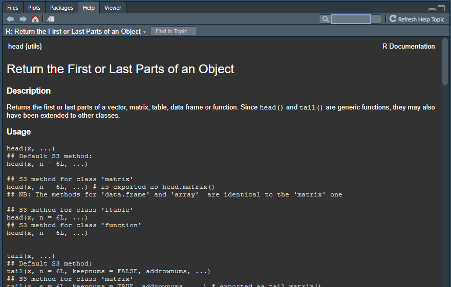
If you are having trouble understanding what a function does or how to use it, you can ask R for help and it will open up a page explaining what the function does, what options it has, and examples of how to use it. To do so we write help(function) or ?function in the console and it will open up that function’s help page. For finding the help page of a function we do not include the parentheses part of the function: help(head) works while help(head()) does not.
If we wrote help(head) to figure out what the head() function does, it will open up this page. Unfortunately, many help pages are not that useful. The following image shows the help page for head(), and it is not very friendly to a new R programmer. In cases where the help page is not useful, and you’re looking at functions not covered in this book, I recommend looking online for help pages dedicated to that function or broader programming sites such as Stack Overflow, where people can ask questions about programming.
For head(), all we need to do is tell the function what data we’re looking at. In programming terms, the input to the function (what we have to include in the parentheses) is the name of our data object. We’ll look at the very commonly used data called mtcars. mtcars is one of a small number of data files that are already in R when you open it. These are included in R just as examples of data to use when testing our code or teaching people to use R. Just type mtcars into the console and it will print out data to the console; there’s nothing you need to do to load the data into R. mtcars has info about a number of cars with each row being a type of car and each column being information about the car such as the miles per gallon it gets and how many gears it has.
We’ll use the head() function to print out just the first 6 rows of the mtcars data.
head(mtcars)
#                    mpg cyl disp  hp drat    wt  qsec vs am gear carb
# Mazda RX4         21.0   6  160 110 3.90 2.620 16.46  0  1    4    4
# Mazda RX4 Wag     21.0   6  160 110 3.90 2.875 17.02  0  1    4    4
# Datsun 710        22.8   4  108  93 3.85 2.320 18.61  1  1    4    1
# Hornet 4 Drive    21.4   6  258 110 3.08 3.215 19.44  1  0    3    1
# Hornet Sportabout 18.7   8  360 175 3.15 3.440 17.02  0  0    3    2
# Valiant           18.1   6  225 105 2.76 3.460 20.22  1  0    3    1
Now we have the first 6 rows of every column from the mtcars data. This is a fairly simple function and is useful for quickly looking at our data. Many functions are more complicated than head() and involve multiple inputs rather than just the single input we had here. Some functions, for example, let you choose how you want the function to operate, as it can do so in multiple ways. Even in head() there’s an optional input to choose how many rows you want it to return, with the default being 6. Since we didn’t choose anything, the function stuck to the default and returned only 6 rows.
Throughout this book we’ll spend a lot of time introducing functions that other people have made and learning how to combine the functions together to be able to get our raw data (e.g. a CSV file downloaded from a police site) into a usable format for research (e.g. cleaned to include only the rows and columns we need to analyze and in the units we want). For functions that other people wrote, we need to tell R that we want to use these functions. We do so by having R download that person’s package. A package is just the name for a collection of functions in an easily downloadable format. We can do all of the downloading through R, so we don’t have to go searching for them. There are two ways to download a package in R: through writing R code or through a shortcut in RStudio.
Downloading a package through R code uses - like pretty much everything else in R - a function. This function is install.packages(), where we put the name of the package we want in the (). This name also has to be in quotes since it is an object that is not currently in R. Let’s install the package “caesar”, which is a simple package I made that creates a Caesar cipher from some text. We need to run the code install.packages("caesar") and be sure to spell “caesar” right and put it in quotes.
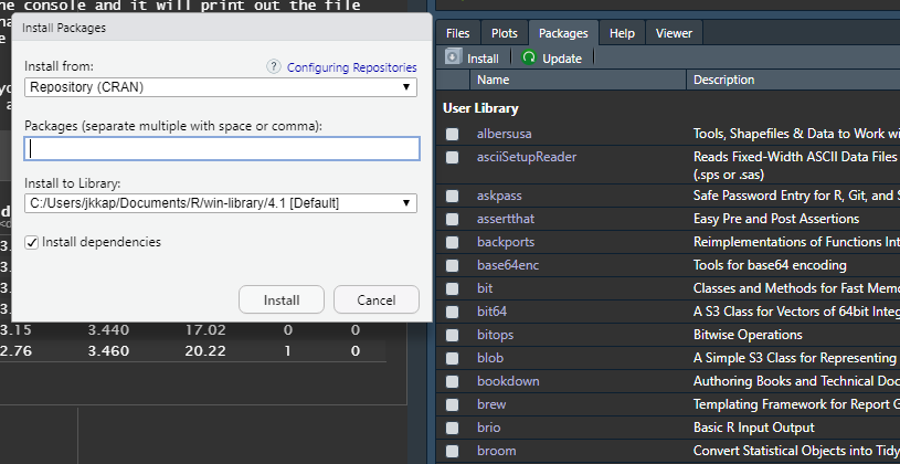
install.packages("caesar")The RStudio shortcut way is to go to the Packages tab and then click Install on the top left of this tab. This will open up a window as shown in the following image where you can enter the name of the package you want. Then click Install and RStudio will install it for you. Also in this tab is the Update button, which allows you to update packages that you have already installed. Since R programmers generally provide updates to their packages (usually bug fixes but occasionally new features and new functions), it’s important to update your packages every several months or so.
Once we have downloaded the package, we need to tell R that we want to use that package. There are thousands of R packages and you’ll likely have hundreds downloaded before long (if a package relies on other packages to work it’ll download those too. So even if you install a single package it may also install other packages necessary for the package you want). Some packages have functions with the same name (but they do different things) so using all packages at once will cause issues since we won’t know which functions we’re actually using. So we only want to use the packages we need for that task. We need a way to tell R that we want to use a package. We only need to do this once per session - that is, once before restarting RStudio. The way to do this is to use the function library(), where we put the package name in the parentheses. Since the package is something that has been installed to R, we don’t need to have quotes around the name.
library(caesar)Now we can run the caesar() function and make a Caesar cipher for that text (it’s just a coincidence that the function name is the same as the package name).
caesar("example text")
# [1] "hAdpsohcwhAw"
2.4 Reading data into R
For many research projects you’ll have data produced by some outside group (e.g. FBI, local police agencies) and you want to take that data and put it inside R to work on it. We call that reading data into R. R is capable of reading a number of different formats of data, which we will discuss in more detail in Chapter 4. Here, we will talk about the standard R data file only.
2.4.1 Loading data
As we learned in Section 2.1.2, we need to set our working directory to the folder where the data is. For my own setup, R is already defaulted to the folder with this data so I do not need to set a working directory. For those following along on your own computer, make sure to set your working directory now.
The load() function lets us load data already in the R format. These files will end in the extension “.rda” or sometimes “.Rda” or “.RData”. Since we are telling R to load a specific file, we need to have that file name in quotes and include the file extension “.rda”. With .rda data, the object inside the .rda file already has a name so we don’t need to assign a name to the data. With other forms of data such as .csv files, we will need to do that as we’ll see in Chapter 4.
In this example (and elsewhere in this book when I load in data), I have all of the data in a folder called “data” in my working directory, which is why I have “data/” before the data name. You do not need this as you should have all of your data directly in your working directory.
load("data/ucr2017.rda")2.5 First steps to exploring data
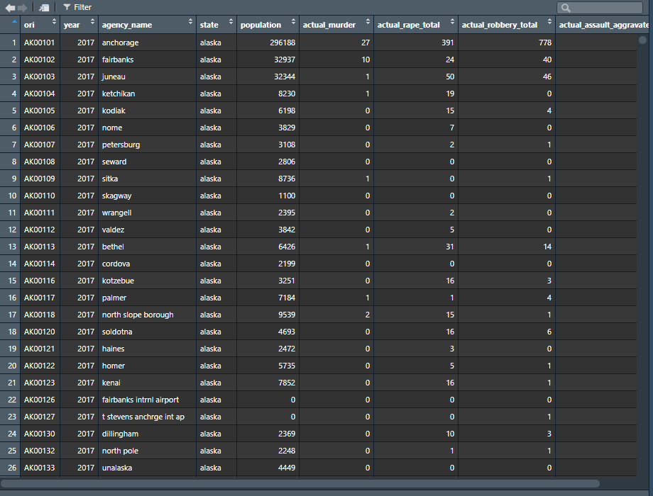
The object we loaded is called ucr2017. We’ll explore this data more thoroughly in Chapter 11, but for now let’s use four simple (and important) functions to get a sense of what the data holds. To use each of these functions, we need to write the name of the data set (without quotes since we don’t need quotes for an object already made in R) inside the ().
head()summary()plot()View()
Note that the first three functions are lowercase while View() is capitalized. That is simply because older functions in R were often capitalized while newer ones use all lowercase letters. R is case sensitive so using view() will not work.
The head() function prints the first 6 rows of each column of the data to the console. This is useful to get a quick glance at the data but has some important drawbacks. When using data with a large number of columns it can be quickly overwhelming by printing too much. There may also be differences in the first 6 rows with other rows. For example, if the rows are ordered chronologically (as is the case with most crime data) the first 6 rows will be the most recent. If data collection methods or the quality of collection changed over time, these 6 rows won’t be representative of the data.
head(ucr2017)
#       ori year agency_name  state population actual_murder actual_rape_total
# 1 AK00101 2017   anchorage alaska     296188            27               391
# 2 AK00102 2017   fairbanks alaska      32937            10                24
# 3 AK00103 2017      juneau alaska      32344             1                50
# 4 AK00104 2017   ketchikan alaska       8230             1                19
# 5 AK00105 2017      kodiak alaska       6198             0                15
# 6 AK00106 2017        nome alaska       3829             0                 7
#   actual_robbery_total actual_assault_aggravated
# 1                  778                      2368
# 2                   40                       131
# 3                   46                       206
# 4                    0                        14
# 5                    4                        41
# 6                    0                        52
The summary() function gives a six-number summary of each numeric or Date column in the data. For other types of data, such as “character” types (which are just columns with words rather than numbers or dates), it’ll say what type of data it is. We’ll cover different types of data in Chapter 3.
The six values it returns for numeric and Date columns are
- The minimum value
- The value at the 1st quartile
- The median value
- The mean value
- The value at the 3rd quartile
- The max value
In cases where there are NAs, it will say how many NAs there are. An NA value is a missing value. Think of it like an empty cell in an Excel file. NA values will cause issues when doing math, such as finding the mean of a column, as R doesn’t know how to handle a NA value in these situations, though summary() automatically excludes NAs when doing the math operations.
summary(ucr2017)
#      ori                 year      agency_name           state
#  Length:15764       Min.   :2017   Length:15764       Length:15764
#  Class :character   1st Qu.:2017   Class :character   Class :character
#  Mode  :character   Median :2017   Mode  :character   Mode  :character
#                     Mean   :2017
#                     3rd Qu.:2017
#                     Max.   :2017
#    population      actual_murder     actual_rape_total  actual_robbery_total
#  Min.   :      0   Min.   :  0.000   Min.   :  -2.000   Min.   :   -1.00
#  1st Qu.:    914   1st Qu.:  0.000   1st Qu.:   0.000   1st Qu.:    0.00
#  Median :   4460   Median :  0.000   Median :   1.000   Median :    0.00
#  Mean   :  19872   Mean   :  1.069   Mean   :   8.262   Mean   :   19.85
#  3rd Qu.:  15390   3rd Qu.:  0.000   3rd Qu.:   5.000   3rd Qu.:    4.00
#  Max.   :8616333   Max.   :653.000   Max.   :2455.000   Max.   :13995.00
#  actual_assault_aggravated
#  Min.   :   -1.00
#  1st Qu.:    1.00
#  Median :    5.00
#  Mean   :   49.98
#  3rd Qu.:   21.00
#  Max.   :29771.00
The plot() function allows us to graph our data. For criminology research we generally want to make scatterplots to show the relationship between two numeric variables, time-series graphs to see how a variable (or variables) change over time, or barplots comparing categorical variables. Here, we’ll make a scatterplot seeing the relationship between a city’s number of murders and their number of aggravated assaults (assault with a weapon or that causes serious bodily injury).
To do so we must specify which column is displayed on the x-axis and which one is displayed on the y-axis. In Section 10.3.1 we’ll talk explicitly about how to select specific columns from our data. For now, all you need to know is to select a column in which you write the data set name followed by a dollar sign $, followed by the column name. Do not include any quotations or spaces (technically spaces can be included but make it a bit harder to read and are against conventional style when writing R code so we’ll exclude them). Inside of plot() we say that “x = ucr2017$actual_murder” so that column goes on the x-axis and “y = ucr2017$actual_assault_aggravated” so aggravated assault goes on the y-axis. And that’s all it takes to make a simple graph.
plot(x = ucr2017$actual_murder, y = ucr2017$actual_assault_aggravated)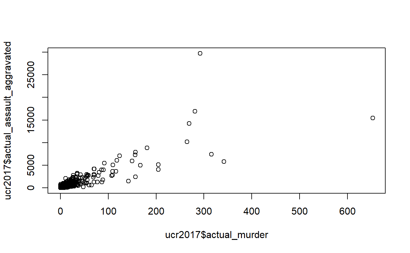
Finally, View() opens essentially an Excel file of the data set you put inside the (). This allows you to look at the data as if it were in Excel (though you can’t edit the data at all here) and is a good way to start to understand the data.
View(ucr2017)