22 Scraping tables from PDFs
For this chapter you’ll need the following file, which is available for download here: usbp_stats_fy2017_sector_profile.pdf.
Government agencies in particular like to release their data in long PDFs which often have the data we want in a table on one of the pages. To use this data we need to scrape it from the PDF into R. In the majority of cases when you want data from a PDF it will be in a table. Essentially the data will be an Excel file inside of a PDF. This format is not altogether different from what we’ve done before.
Let’s first take a look at the data we will be scraping. The first step in any PDF scraping should be to look at the PDF and try to think about the best way to approach this particular problem. While all PDF scraping follows a general format, you cannot necessarily reuse your old code as each situation is likely slightly different. Our data is from the US Customs and Border Protection (CBP) and contains a wealth of information about apprehensions and contraband seizures in border sectors.
We will be using the Sector Profile 2017 PDF which has information in four tables, three of which we’ll scrape and then combine together. The data was downloaded from the US Customs and Border Protection “Stats and Summaries” page here. If you’re interested in using more of their data, some of it has been cleaned and made available here.
The file we want to use is called “usbp_stats_fy2017_sector_profile.pdf” and has four tables in the PDF. Let’s take a look at them one at a time, understanding what variables are available, and what units each row is in. Then we’ll start scraping the tables.
The first table is “Sector Profile - Fiscal Year 2017 (Oct. 1st through Sept. 30th)”. Before we even look down more at the table, the title is important. It is for fiscal year 2017, not calendar year 2017, which is more common in the data we usually use. This is important if we ever want to merge this data with other data sets. If possible, we would have to get data that is monthly so we can just use October 2016 through September 2017 to match up properly.
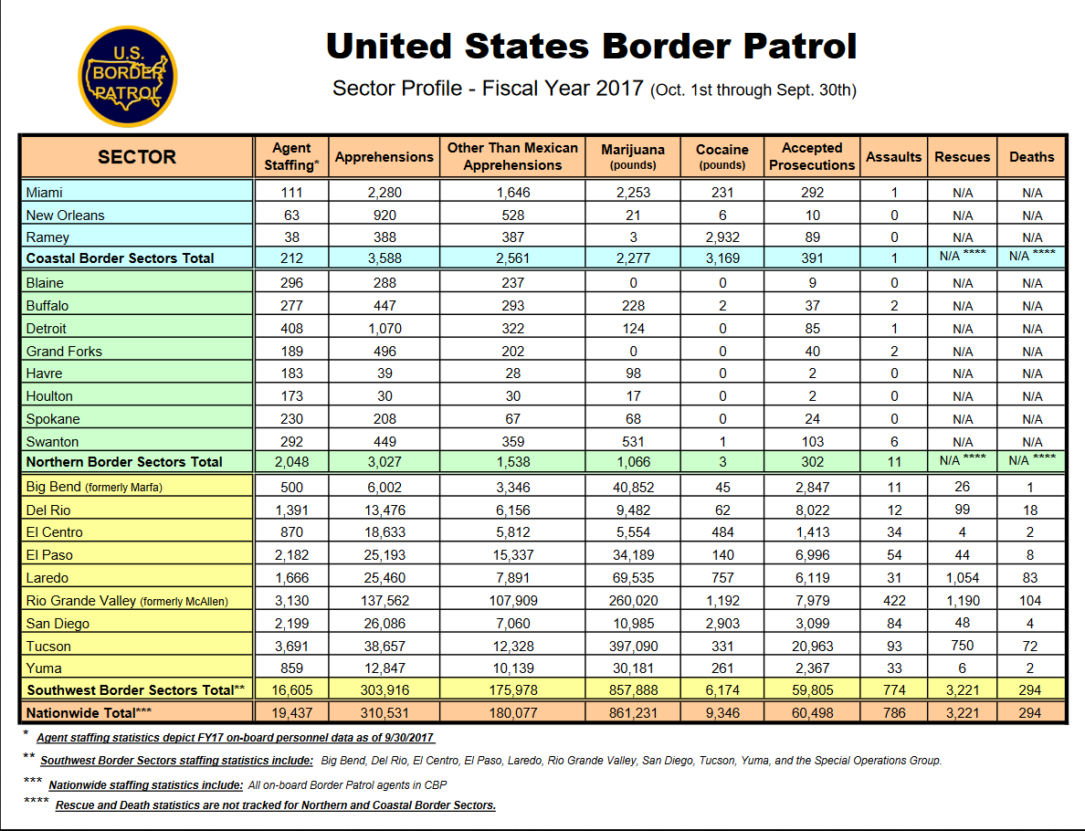
Now if we look more at the table, we can see that each row is a section of the US border. There are three main sections - Coastal, Northern, and Southwest, with subsections of each also included. The bottom row is the sum of all these sections and gives us nationwide data. Many government data sets will be like this form with sections and subsections in the same table. Watch out when doing mathematical operations! Just summing any of these columns will give you triple the true value due to the presence of nationwide, sectional, and subsectional data.
There are 9 columns in the data other than the border section identifier. We have total apprehensions, apprehensions for people who are not Mexican citizens, marijuana and cocaine seizures (in pounds), the number of accepted prosecutions (presumably of those apprehended), and the number of CBP agents assaulted. The last two columns have the number of people rescued by CBP and the number of people who died (it is unclear from this data alone if this is solely people in custody or deaths during crossing the border). These two columns are also special as they only have data for the Southwest border.
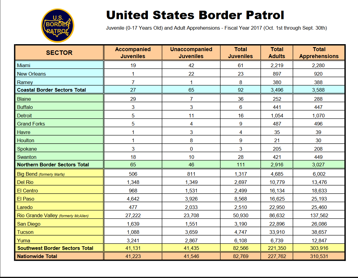
The second table has a similar format with each row being a section or subsection. The columns now have the number of juveniles apprehended, subdivided by if they were accompanied by an adult or not, and the number of adults apprehended. The last column is total apprehensions which is also in the first table.
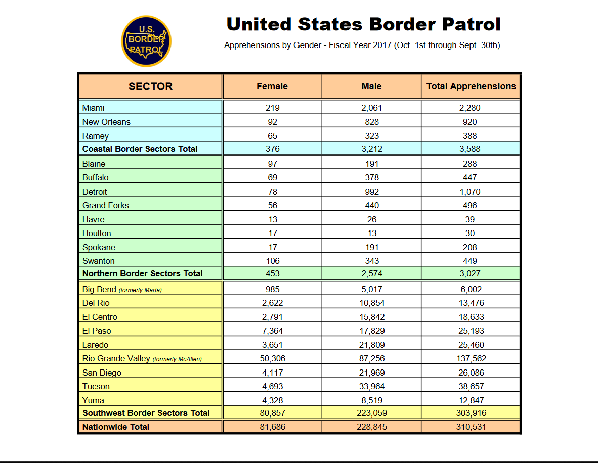
The third table follows the same format, and the new columns are number of apprehensions by gender.
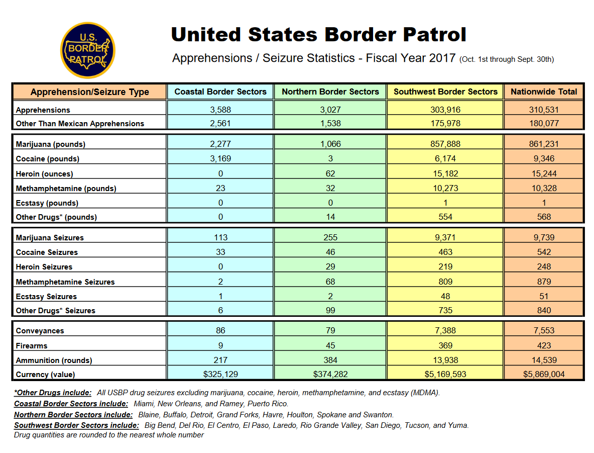
Finally, the fourth table is a bit different in its format. The rows are now variables, and the columns are the locations. In this table it doesn’t include subsections, only border sections and the nationwide total. The data it has available are partially a repeat of the first table but with more drug types and the addition of the number of drug seizures and some firearm seizure information. As this table is formatted differently from the others, we won’t scrape it in this lesson - but you can use the skills you’ll learn to do so yourself.
22.1 Scraping the first table
We’ve now seen all three of the tables that we want to scrape so we can begin the process of actually scraping them. Note that each table is very similar, meaning that we can reuse some code to scrape as well as to clean the data. That means that we will want to write some functions to make our work easier and avoid copy and pasting code.
We will start by using the pdf_text() function from the pdftools package to read the PDFs into R.
install.packages("pdftools")library(pdftools)
# Using poppler version 22.04.0We can assign the output of the pdf_text() function to the object border_patrol, and we’ll use it for each table. The input to pdf_text() is the name of the PDF we want to scrape.
border_patrol <- pdf_text("data/usbp_stats_fy2017_sector_profile.pdf")We can take a look at the head() of the result using head(border_patrol).
head(border_patrol)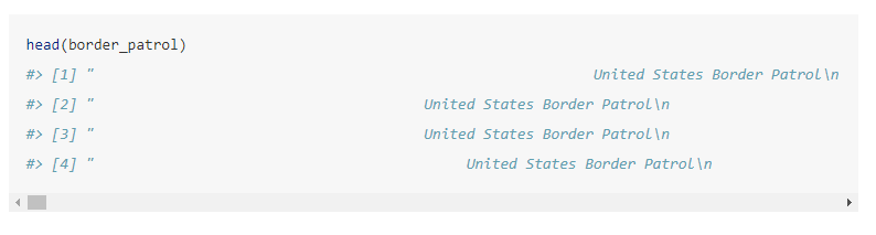
If you look closely in this huge amount of text output, you can see that it is a vector with each table being an element in the vector. We can see this further by checking the length() of “border_patrol”, which tells us how many elements are in a vector.
length(border_patrol)
# [1] 4
It is four elements long, one for each table.
Looking at just the first element in border_patrol gives us all the values in the first table plus a few sentences at the end detailing some features of the table. At the end of each line (where in the PDF it should end but doesn’t in our data yet) there is a \n indicating that there should be a new line. We want to use strsplit() to split at the \n.
border_patrol[1]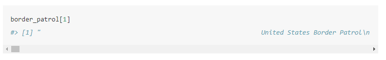
The strsplit() function breaks up a string into pieces based on a value inside of the string. Let’s use the word “criminology” as an example. If we want to split it by the letter “n” we’d have two results, “crimi” and “ology” as these are the pieces of the word after breaking up “criminology” at letter “n”.
strsplit("criminology", split = "n")
# [[1]]
# [1] "crimi" "ology"
Note that it deletes whatever value is used to break up the string.
Let’s assign a new object with the value in the first element of border_patrol, calling it sector_profile as that’s the name of that table, and then using strsplit() on it to split it every \n. In effect this makes each line of the table an element in a vector that we’ll create rather than having the entire table be a single long string as it is now. strsplit() returns a list so we will also want to keep just the first element of that list using double square bracket [[]] notation.
sector_profile <- border_patrol[1]
sector_profile <- strsplit(sector_profile, "\n")
sector_profile <- sector_profile[[1]]
Now we can look at the first six rows of this data.
head(sector_profile)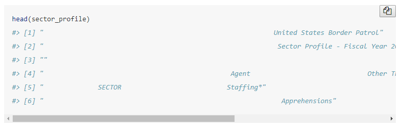
Notice that there is a lot of empty white space at the beginning of the rows. We want to get rid of that to make our next steps easier. We can use trimws() and put the entire sector_profile data in the (), and it’ll remove any white space that is at the beginning or end of the string.
sector_profile <- trimws(sector_profile)We have more rows than we want so let’s look at the entire data and try to figure out how to keep just the necessary rows.
sector_profile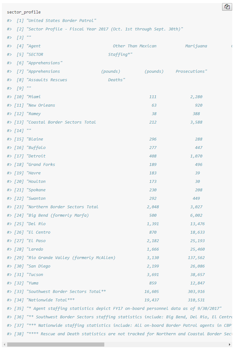
Based on the PDF, we want every row from Miami to Nationwide Total. But here we have several rows with the title of the table and the column names, and at the end we have the sentences with some details that we don’t need.
To keep only the rows that we want, we can combine grep() and subsetting to find the rows from Miami to Nationwide Total and keep only those rows. We will use grep() to find which row has the text “Miami” and which has the text “Nationwide Total” and keep all rows between them (including those matched rows as well). Since each only appears once in the table we don’t need to worry about handling duplicate results.
grep("Miami", sector_profile)
# [1] 10grep("Nationwide Total", sector_profile)
# [1] 35We’ll use square bracket notation to keep all rows between those two values (including each value). Since the data is a vector, not a data.frame, we don’t need a comma.
sector_profile <- sector_profile[grep("Miami", sector_profile):
                                   grep("Nationwide Total", sector_profile)]
Note that we’re getting rid of the rows that had the column names. It’s easier to make the names ourselves than to deal with that mess. The data now has only the rows we want but still doesn’t have any columns, it’s currently just a vector of strings. We want to make it into a data.frame to be able to work on it like we usually do.
head(sector_profile)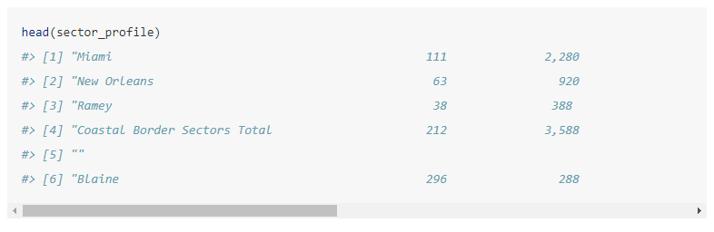
When looking at this data it is clear that where the division between columns is supposed to be is a bunch of white space in each string. Take the first row for example, it says “Miami” then after lots of white spaces “111” than again with “2,280” and so on for the rest of the row. We’ll use this pattern of columns differentiated by white space to make sector_profile into a data.frame.
We will use the function str_split_fixed() from the stringr package. This function is very similar to strsplit() except you can tell it how many columns to expect.
install.packages("stringr")library(stringr)
# Warning: package 'stringr' was built under R version 4.2.2The syntax of str_split_fixed() is similar to strsplit() except the new parameter of the number of splits to expect. The “_fixed” part of str_split_fixed() is that it expects the same number of splits (which in our case become columns) for every element in the vector that we input. Looking at the PDF shows us that there are 10 columns so that’s the number we’ll use. Our split will be ” {2,}“. That is, a space that occurs two or more times. Since there are sectors with spaces in their name, we can’t have only one space, we need at least two. If you look carefully at the rows with sectors”Coastal Border Sectors Total” and “Northern Border Sectors Total”, the final two columns actually do not have two spaces between them because of the amount of asterisks they have. Normally we’d want to fix this using gsub(), but those values will turn to NA anyway so we won’t bother in this case.
sector_profile <- str_split_fixed(sector_profile, " {2,}", 10)If we check the head() we can see that we have the proper columns now, but this still isn’t a data.frame and has no column names.
head(sector_profile)
#      [,1]                           [,2]  [,3]    [,4]
# [1,] "Miami"                        "111" "2,280" "1,646"
# [2,] "New Orleans"                  "63"  "920"   "528"
# [3,] "Ramey"                        "38"  "388"   "387"
# [4,] "Coastal Border Sectors Total" "212" "3,588" "2,561"
# [5,] ""                             ""    ""      ""
# [6,] "Blaine"                       "296" "288"   "237"
#      [,5]    [,6]    [,7]  [,8] [,9]       [,10]
# [1,] "2,253" "231"   "292" "1"  "N/A"      "N/A"
# [2,] "21"    "6"     "10"  "0"  "N/A"      "N/A"
# [3,] "3"     "2,932" "89"  "0"  "N/A"      "N/A"
# [4,] "2,277" "3,169" "391" "1"  "N/A ****" "N/A ****"
# [5,] ""      ""      ""    ""   ""         ""
# [6,] "0"     "0"     "9"   "0"  "N/A"      "N/A"
We can make it a data.frame just by putting it in data.frame(). And we can assign the columns names using a vector of strings we can make. We’ll use the same column names as in the PDF but in lowercase and replacing spaces and parentheses with underscores.
sector_profile <- data.frame(sector_profile)
names(sector_profile) <- c("sector",
                           "agent_staffing",
                           "apprehensions",
                           "other_than_mexican_apprehensions",
                           "marijuana_pounds",
                           "cocaine_pounds",
                           "accepted_prosecutions",
                           "assaults",
                           "rescues",
                           "deaths")
We have now taken a table from a PDF and successfully scraped it to a data.frame in R. Now we can work on it as we would any other data set that we’ve used previously.
head(sector_profile)
#                         sector agent_staffing apprehensions
# 1                        Miami            111         2,280
# 2                  New Orleans             63           920
# 3                        Ramey             38           388
# 4 Coastal Border Sectors Total            212         3,588
# 5
# 6                       Blaine            296           288
#   other_than_mexican_apprehensions marijuana_pounds
# 1                            1,646            2,253
# 2                              528               21
# 3                              387                3
# 4                            2,561            2,277
# 5
# 6                              237                0
#   cocaine_pounds accepted_prosecutions assaults  rescues
# 1            231                   292        1      N/A
# 2              6                    10        0      N/A
# 3          2,932                    89        0      N/A
# 4          3,169                   391        1 N/A ****
# 5
# 6              0                     9        0      N/A
#     deaths
# 1      N/A
# 2      N/A
# 3      N/A
# 4 N/A ****
# 5
# 6      N/A
To really be able to use this data we’ll want to clean the columns to turn the values to numeric type, but we can leave that until later. For now let’s write a function that replicates much of this work for the next tables.
22.2 Making a function
As we’ve done before, we want to take the code we wrote for the specific case of the first table in this PDF and turn it into a function for the general case of other tables in the PDF. Let’s copy the code we used previously before we convert it to a function.
sector_profile <- border_patrol[1]
sector_profile <- trimws(sector_profile)
sector_profile <- strsplit(sector_profile, "\r\n")
sector_profile <- sector_profile[[1]]
sector_profile <- sector_profile[grep("Miami",
                                      sector_profile):
                                   grep("Nationwide Total",
                                        sector_profile)]
sector_profile <- str_split_fixed(sector_profile, " {2,}", 10)
sector_profile <- data.frame(sector_profile)
names(sector_profile) <- c("sector",
                           "agent_staffing",
                           "total_apprehensions",
                           "other_than_mexican_apprehensions",
                           "marijuana_pounds",
                           "cocaine_pounds",
                           "accepted_prosecutions",
                           "assaults",
                           "rescues",
                           "deaths")
Since each table is so similar our function will only need a few changes in the above code to work for all three tables. The object border_patrol has all four of the tables in the data, so we need to say which of these tables we want - we can call the parameter table_number. Then each table has a different number of columns so we need to change the str_split_fixed() function to take a variable with the number of columns we input, a value we’ll call number_columns. We rename each column to its proper name so we need to input a vector - which we’ll call column_names - with the names for each column. Finally, we want to have a parameter where we enter in the data, which holds all of the tables, our object border_patrol, we can call this list_of_tables as it is fairly descriptive.
We do this as it is bad form (and potentially dangerous) to have a function that relies on an object that isn’t explicitly put in the function. It we change our border_patrol object (such as by scraping a different file but calling that object border_patrol) and the function doesn’t have that as an input, it will work differently than we expect. Since we called the object we scraped sector_profile for the first table, let’s change that to data as not all tables are called Sector Profile.
scrape_pdf <- function(list_of_tables,
                       table_number,
                       number_columns,
                       column_names) {
  data <- list_of_tables[table_number]
  data <- trimws(data)
  data <- strsplit(data, "\n")
  data <- data[[1]]
  data <- data[grep("Miami", data):
                 grep("Nationwide Total", data)]
  data <- str_split_fixed(data, " {2,}", number_columns)
  data <- data.frame(data)
  names(data) <- column_names

  return(data)
}
Now let’s run this function for each of the three tables we want to scrape, changing the function’s parameters to work for each table. To see what parameter values you need to input, look at the PDF itself or the screenshots in this lesson.
table_1 <- scrape_pdf(list_of_tables = border_patrol,
                      table_number = 1,
                      number_columns = 10,
                      column_names = c("sector",
                                       "agent_staffing",
                                       "total_apprehensions",
                                       "other_than_mexican_apprehensions",
                                       "marijuana_pounds",
                                       "cocaine_pounds",
                                       "accepted_prosecutions",
                                       "assaults",
                                       "rescues",
                                       "deaths"))
table_2 <- scrape_pdf(list_of_tables = border_patrol,
                      table_number = 2,
                      number_columns = 6,
                      column_names = c("sector",
                                       "accompanied_juveniles",
                                       "unaccompanied_juveniles",
                                       "total_juveniles",
                                       "total_adults",
                                       "total_apprehensions"))
table_3 <- scrape_pdf(list_of_tables = border_patrol,
                      table_number = 3,
                      number_columns = 4,
                      column_names = c("sector",
                                       "female",
                                       "male",
                                       "total_apprehensions"))
We can use the function left_join() from the dplyr package to combine the three tables into a single object. In the first table there are some asterisks after the final two row names in the Sector column. For our match to work properly we need to delete them, which we can do using gsub().
table_1$sector <- gsub("\\*", "", table_1$sector)Now we can run left_join(). left_join() will automatically join based on shared column names in the two data sets we are joining. In our case this is “sector” and “total_apprehensions.” All we need to input into left_join() is the name of the data sets we want to join together. left_join() can only combine two data sets at a time so we’ll first join table_1 and table_2 and then join table_3 with the result of the first join, which we’ll call “final_data.”
library(dplyr)
#
# Attaching package: 'dplyr'
# The following objects are masked from 'package:stats':
#
#     filter, lag
# The following objects are masked from 'package:base':
#
#     intersect, setdiff, setequal, union
final_data <- left_join(table_1, table_2)
# Joining, by = c("sector", "total_apprehensions")
final_data <- left_join(final_data, table_3)
# Joining, by = c("sector", "total_apprehensions")
Let’s take a look at the head() of this combined data.
head(final_data)
#                         sector agent_staffing
# 1                        Miami            111
# 2                  New Orleans             63
# 3                        Ramey             38
# 4 Coastal Border Sectors Total            212
# 5
# 6                       Blaine            296
#   total_apprehensions other_than_mexican_apprehensions
# 1               2,280                            1,646
# 2                 920                              528
# 3                 388                              387
# 4               3,588                            2,561
# 5
# 6                 288                              237
#   marijuana_pounds cocaine_pounds accepted_prosecutions
# 1            2,253            231                   292
# 2               21              6                    10
# 3                3          2,932                    89
# 4            2,277          3,169                   391
# 5
# 6                0              0                     9
#   assaults  rescues   deaths accompanied_juveniles
# 1        1      N/A      N/A                    19
# 2        0      N/A      N/A                     1
# 3        0      N/A      N/A                     7
# 4        1 N/A **** N/A ****                    27
# 5                                             <NA>
# 6        0      N/A      N/A                    29
#   unaccompanied_juveniles total_juveniles total_adults
# 1                      42              61        2,219
# 2                      22              23          897
# 3                       1               8          380
# 4                      65              92        3,496
# 5                    <NA>            <NA>         <NA>
# 6                       7              36          252
#   female  male
# 1    219 2,061
# 2     92   828
# 3     65   323
# 4    376 3,212
# 5   <NA>  <NA>
# 6     97   191
In one data set we now have information from three separate tables in a PDF. We have now scraped three different tables from a PDF and turned them into a single data set, turning the PDF into actually usable (and useful) data!