24 Geocoding
For this chapter you’ll need the following file, which is available for download here: san_francisco_active_marijuana_retailers.csv.
Several recent studies have looked at the effect of marijuana dispensaries on crime around the dispensary. For these analyses they find the coordinates of each crime in the city and see if it occurred in a certain distance from the dispensary. Many crime data sets provide the coordinates of where each crime occurred, however sometimes the coordinates are missing - and other data such as marijuana dispensary locations give only the address - meaning that we need a way to find the coordinates of these locations.
24.1 Geocoding a single address
In this chapter we will cover how to geocode addresses. Geocoding is the process of taking an address (e.g. 123 Main Street, Somewhere, CA, 12345) and getting the longitude and latitude coordinates of that address. With these coordinates we can then do spatial analyses on the data ranging from simply making a map and showing where each address is to merging these coordinates with some other spatial data (such as seeing which police district the address is in) and seeing how it relates to other variables, such as crime.
To do our geocoding, we’re going to use the package tidygeocoder which greatly simplifies the work of geocoding addresses in R. For more information about this package, please see the package’s site here. If you’ve never used this package before you’ll need to install it using install.packages("tidygeocoder").
install.packages("tidygeocoder")Now we need to tell R that we want to use this package by running library(tidygeocoder).
library(tidygeocoder)To geocode our addresses we’ll use the helpfully named geocode() function inside of tidygeocoder. For geocode() we input an address and it returns the coordinates for that address. For our address we’ll use “750 Race St. Philadelphia, PA 19106,” which is the address of the Philadelphia Police Department headquarters.
geocode("750 Race St. Philadelphia, PA 19106")
# Error: .tbl is not a dataframe. See ?geocode
As shown above, running geocode("750 Race St. Philadelphia, PA 19106") gives us an error that tells us that “.tbl is not a dataframe.” The issue is that geocode() expects a data.frame (and .tbl is an abbreviation for tibble, which is a kind of data.frame), but we entered only the string with our one address, not a data.frame. For this function to work we need to enter two parameters into geocode(): a data.frame (or something similar such as a tibble) and the name of the column that has the addresses.22 Since we need a data.frame, we’ll make one below. I’m calling it address_to_geocode and calling the column with the address “address”, but you can call both the data.frame and the column whatever name you want.
address_to_geocode <- data.frame(address =
                      "750 Race St. Philadelphia, PA 19106")
Now let’s try again. We’ll enter our data.frame address_to_geocode first and then the name of our column which is “address”.
geocode(address_to_geocode, address)
# # A tibble: 1 × 3
#   address                               lat  long
#   <chr>                               <dbl> <dbl>
# 1 750 Race St. Philadelphia, PA 19106  40.0 -75.2
It worked, returning the same data.frame but with two additional columns with the latitude and longitude of that address.
You might be wondering why we put “address” into geocode() without quotes when usually when we talk about a column we need to do so in quotes. The simple answer is that the authors of the tidygeocoder package spent the time allowing users to input the column name either with or without quotes. Trying it again and now having “address” in quotes gives us the same result.
geocode(address_to_geocode, "address")
# # A tibble: 1 × 3
#   address                               lat  long
#   <chr>                               <dbl> <dbl>
# 1 750 Race St. Philadelphia, PA 19106  40.0 -75.2
There are two additional parameters that are important to talk about for this function, especially when you encounter an address that doesn’t geocode properly.
First, there are actually multiple sources where you can enter an address and get the coordinates for that address. Just think about the big mapping apps or sites, such as Google Maps and Apple Maps. For these sources you can enter in the same address and you’ll get different results. In most cases you’ll get extremely similar coordinates, usually off only after a few decimals points, so they are functionally identical. But occasionally you’ll have some addresses that can be geocoded through some sources but not others. This is because some sources have a more comprehensive list of addresses than others.
At the time of this writing the tidygeocoder package can handle geocoding from 13 different sources. For 10 of these, however, you need to setup an API key and some also require paying money (usually after a set number of addresses that it’ll geocode for free each day). So here I’ll just cover the three sources of geocoding that don’t require any setup: “osm” (Open Street Map or OSM is similar to Google Maps), “census” (the US Census Bureau’s geocoder), and “arcgis” (ArcGIS is a clunky mapping software that nonetheless has an excellent geocoder that R can use). To select which of these to use (“osm” is the default), you add the parameter “method” and set that equal to which one you want to use. As “osm” is the default we actually don’t need to set it explicitly, but we’ll do so anyways here as an example of the three geocoding sources we want to use.
example <- geocode(address_to_geocode, "address", method = "osm")
example
# # A tibble: 1 × 3
#   address                               lat  long
#   <chr>                               <dbl> <dbl>
# 1 750 Race St. Philadelphia, PA 19106  40.0 -75.2
example <- geocode(address_to_geocode, "address", method = "census")
example
# # A tibble: 1 × 3
# address lat long
# <chr> <dbl> <dbl>
# 1 750 Race St. Philadelphia, PA 19106 40.0 -75.2example <- geocode(address_to_geocode, "address", method = "arcgis")
example
# # A tibble: 1 × 3
# address lat long
# <chr> <dbl> <dbl>
# 1 750 Race St. Philadelphia, PA 19106 40.0 -75.2By default this function returns a tibble instead of a normal data.frame so it only shows one decimal point by default - though it doesn’t actually round the number, merely shorten what it shows us. We can change the output back into a data.frame by using the data.frame() function. If you check each result after converting it to a data.frame you’ll see that each set of coordinates are very slightly different, though for all purposes are the same location.
example <- geocode(address_to_geocode, "address", method = "arcgis")
example <- data.frame(example)
example
#                               address      lat      long
# 1 750 Race St. Philadelphia, PA 19106 39.95488 -75.15205
Given how similar the coordinates are, you really only need to set the source of the geocoder in cases where one geocoder fails to find a match for the address.
The second important parameter is full_results, which is by default set to FALSE. When set to TRUE it gives more columns in the returning data.frame than just the longitude and latitude of that address. These columns differ for each geocoder source so we’ll look at all three. I’ll convert all of these results to a data.frame so it prints out all of the columns, and doesn’t abbreviate results, which is how tibbles function. The example$display_name <- NULL isn’t necessary, but I use it to remove a column that prints out an extremely long line for the location’s full address and that looks bad in the print version of this book.
example <- geocode(address_to_geocode, "address",
                   method = "osm", full_results = TRUE)
example <- data.frame(example)
example$display_name <- NULL
example
#                               address      lat      long  place_id
# 1 750 Race St. Philadelphia, PA 19106 39.95506 -75.15217 304083147
#                                                                  licence
# 1 Data © OpenStreetMap contributors, ODbL 1.0. https://osm.org/copyright
#   osm_type    osm_id
# 1      way 626341043
#                                                            boundingbox class
# 1 39.955010747193, 39.955110747193, -75.152217431613, -75.152117431613 place
#    type importance
# 1 house      -0.62
For OSM as a source we also get information about the address, such as what type of place it is, a bounding box which is a geographic area right around this coordinate, the address for those coordinates in the OSM database, and a bunch of other variables that don’t seem very useful for our purposes such as the “importance” of the address. It’s interesting that OSM classifies this address as a “house” as the headquarters of a major police department is quite a bit bigger than a house, so this is likely an misclassification of the type of address. The most important extra variable here is the address, called the “display_name”.
Sometimes geocoders will be quite a bit off in their geocoding because they match the address you inputted incorrectly to one in their database. For example, if you input “123 Main Street” and the geocoder thinks you mean “123 Maine Street” you may be quite a bit off in the resulting coordinates. When you only get coordinates returned you won’t know that the coordinates are wrong. Even if you know where an address is supposed to be it’s hard to catch errors like this. If you’re geocoding addresses in a single city and one point is in a different city (or completely different part of the world), then it’s pretty clear that there’s an error. But if the coordinates are simply in a wrong part of the city, but near other coordinates, then it’s very hard to notice a problem. So having an address to check against the one you inputted is a very useful way of validate the geocoding.
example <- geocode(address_to_geocode, "address",
                   method = "census", full_results = TRUE)
example <- data.frame(example)
example
#                               address      lat     long
# 1 750 Race St. Philadelphia, PA 19106 39.95488 -75.1514
#                         matchedAddress tigerLine.side tigerLine.tigerLineId
# 1 750 RACE ST, PHILADELPHIA, PA, 19106              L             131423677
#   addressComponents.zip addressComponents.streetName addressComponents.preType
# 1                 19106                         RACE
#   addressComponents.city addressComponents.preDirection
# 1           PHILADELPHIA
#   addressComponents.suffixDirection addressComponents.fromAddress
# 1                                                             700
#   addressComponents.state addressComponents.suffixType
# 1                      PA                           ST
#   addressComponents.toAddress addressComponents.suffixQualifier
# 1                         798
#   addressComponents.preQualifier
# 1
The Census results are similar to the OSM results and also have the matched address to compare your inputted address to. Most of the columns are just the address broken into different pieces (street, city, state, etc.) so are mostly repeating the address again in multiple columns.
example <- geocode(address_to_geocode, "address",
                   method = "arcgis", full_results = TRUE)
example <- data.frame(example)
example
#                               address      lat      long
# 1 750 Race St. Philadelphia, PA 19106 39.95488 -75.15205
#                                   arcgis_address score location.x location.y
# 1 750 Race St, Philadelphia, Pennsylvania, 19106   100  -75.15205   39.95488
#   extent.xmin extent.ymin extent.xmax extent.ymax
# 1   -75.15305    39.95388   -75.15105    39.95588
For the ArcGIS results we have the matched address again, and then an important variable called “score,” which is basically a measure of how confident ArcGIS is that it matched the right address. Higher values are more confident, but in my experience anything under 90-95 confidence is an incorrect address. These results also repeat the longitude and latitude columns as “location.x” and “location.y” columns, and I’m not sure why they do so.
24.2 Geocoding San Francisco marijuana dispensary locations
So now that we can use the geocoder() function well, we can geocode every location in our marijuana dispensary data.
Let’s read in the marijuana dispensary data, which is called “san_francisco_active_marijuana_retailers.csv” and call the object marijuana. Note the “data/” part in front of the name of the .csv file. This is to tell R that the file we want is in the “data” folder of our working directory. Doing this is essentially a shortcut to changing the working directory directly. For this book I keep all of the data files in a folder called “data” in my working directory. Unless you also have a folder called “data” in your working directory which has this file, please delete “data/” from the following code.
library(readr)
marijuana <- read_csv("data/san_francisco_active_marijuana_retailers.csv")
marijuana <- data.frame(marijuana)
Let’s look at the top 6 rows.
head(marijuana)
#    License.Number                License.Type   Business.Owner
# 1 C10-0000614-LIC Cannabis - Retailer License     Terry Muller
# 2 C10-0000586-LIC Cannabis - Retailer License    Jeremy Goodin
# 3 C10-0000587-LIC Cannabis - Retailer License     Justin Jarin
# 4 C10-0000539-LIC Cannabis - Retailer License Ondyn Herschelle
# 5 C10-0000522-LIC Cannabis - Retailer License      Ryan Hudson
# 6 C10-0000523-LIC Cannabis - Retailer License      Ryan Hudson
#          Business.Structure
# 1 Limited Liability Company
# 2               Corporation
# 3               Corporation
# 4               Corporation
# 5 Limited Liability Company
# 6 Limited Liability Company
#                                                 Premise.Address Status
# 1  2165 IRVING ST san francisco, CA 94122 County: SAN FRANCISCO Active
# 2 122 10TH ST SAN FRANCISCO, CA 941032605 County: SAN FRANCISCO Active
# 3   843 Howard ST SAN FRANCISCO, CA 94103 County: SAN FRANCISCO Active
# 4    70 SECOND ST SAN FRANCISCO, CA 94105 County: SAN FRANCISCO Active
# 5   527 Howard ST San Francisco, CA 94105 County: SAN FRANCISCO Active
# 6 2414 Lombard ST San Francisco, CA 94123 County: SAN FRANCISCO Active
#   Issue.Date Expiration.Date                Activities Adult.Use.Medicinal
# 1  9/13/2019       9/12/2020 N/A for this license type                BOTH
# 2  8/26/2019       8/25/2020 N/A for this license type                BOTH
# 3  8/26/2019       8/25/2020 N/A for this license type                BOTH
# 4   8/5/2019        8/4/2020 N/A for this license type                BOTH
# 5  7/29/2019       7/28/2020 N/A for this license type                BOTH
# 6  7/29/2019       7/28/2020 N/A for this license type                BOTH
The column with the address is called Premise Address. Since the address county is always “County: SAN FRANCISCO” we can just gsub() out that entire string.
marijuana$Premise.Address <- gsub(" County: SAN FRANCISCO",
                                  "", marijuana$Premise.Address)
Now let’s make sure we did it right.
head(marijuana$Premise.Address)
# [1] "2165 IRVING ST san francisco, CA 94122"
# [2] "122 10TH ST SAN FRANCISCO, CA 941032605"
# [3] "843 Howard ST SAN FRANCISCO, CA 94103"
# [4] "70 SECOND ST SAN FRANCISCO, CA 94105"
# [5] "527 Howard ST San Francisco, CA 94105"
# [6] "2414 Lombard ST San Francisco, CA 94123"
To do the geocoding we’ll just tell geocode() our data.frame name and the name of the column with the addresses. We’ll assign the results back into the marijuana object. As noted earlier, we don’t need to put the name of our column in quotes, but I like to do so because it is consistent with some other functions that require it. Running this code may take up to a minute because it’s geocoding 33 different addresses.
marijuana <- geocode(marijuana, "Premise.Address")Now it appears that we have longitude and latitude for every dispensary. We should check that they all look sensible.
summary(marijuana$long)
#    Min. 1st Qu.  Median    Mean 3rd Qu.    Max.    NA's
# -122.5 -122.4 -122.4 -122.4 -122.4 -122.4 10summary(marijuana$lat)
# Min. 1st Qu. Median Mean 3rd Qu. Max. NA's
# 37.71 37.75 37.78 37.77 37.78 37.80 10The minimum and maximum are very similar to each other for both longitude and latitude so that’s a sign that it geocoded correctly. The 10 NA values mean that it didn’t find a match for 10 of the addresses. Let’s try again and now set method to “arcgis.” which generally has a very high match rate. Before we do this let’s just remove the entire latitude and longitude columns from our data. How the geocode() function works is that if we keep the “long” and “lat” columns that are currently in the data from when we just geocoded, when we run it again it’ll make new columns that have nearly identical names. We usually want as few columns in our data as possible so there’s no point having the “lat” column from the last geocode run with the 10 NAs and another “lat” (though slightly different, automatically chosen name) column from this time we run geocode().
We could also just geocode the 10 addresses that failed on the first run, but given that we’ll only be geocoding a small number of addresses it won’t take much extra time to have ArcGIS run it all. Running this function on just the NA rows requires a bit more work than just rerunning them all. In general, when the choice is between you spending time writing code and letting the computer do more work, let the computer do the work. And in general I’d recommend starting with ArcGIS as it is more reliable for geocoding. We’ll remove the current coordinate columns by setting them each to NULL.
marijuana$long <- NULL
marijuana$lat  <- NULL
marijuana      <- geocode(marijuana, "Premise.Address",
                          method = "arcgis")
And let’s do the summary() check again.
summary(marijuana$long)
#    Min. 1st Qu.  Median    Mean 3rd Qu.    Max.
# -122.5 -122.4 -122.4 -122.4 -122.4 -122.4summary(marijuana$lat)
# Min. 1st Qu. Median Mean 3rd Qu. Max.
# 37.71 37.76 37.77 37.77 37.78 37.80No more NAs, which means that we successfully geocoded our addresses. Another check is to make a simple scatterplot of the data. Since all of the data is from San Francisco, they should be relatively close to each other. If there are dots far from the rest, that is probably a geocoding issue.
plot(marijuana$long, marijuana$lat)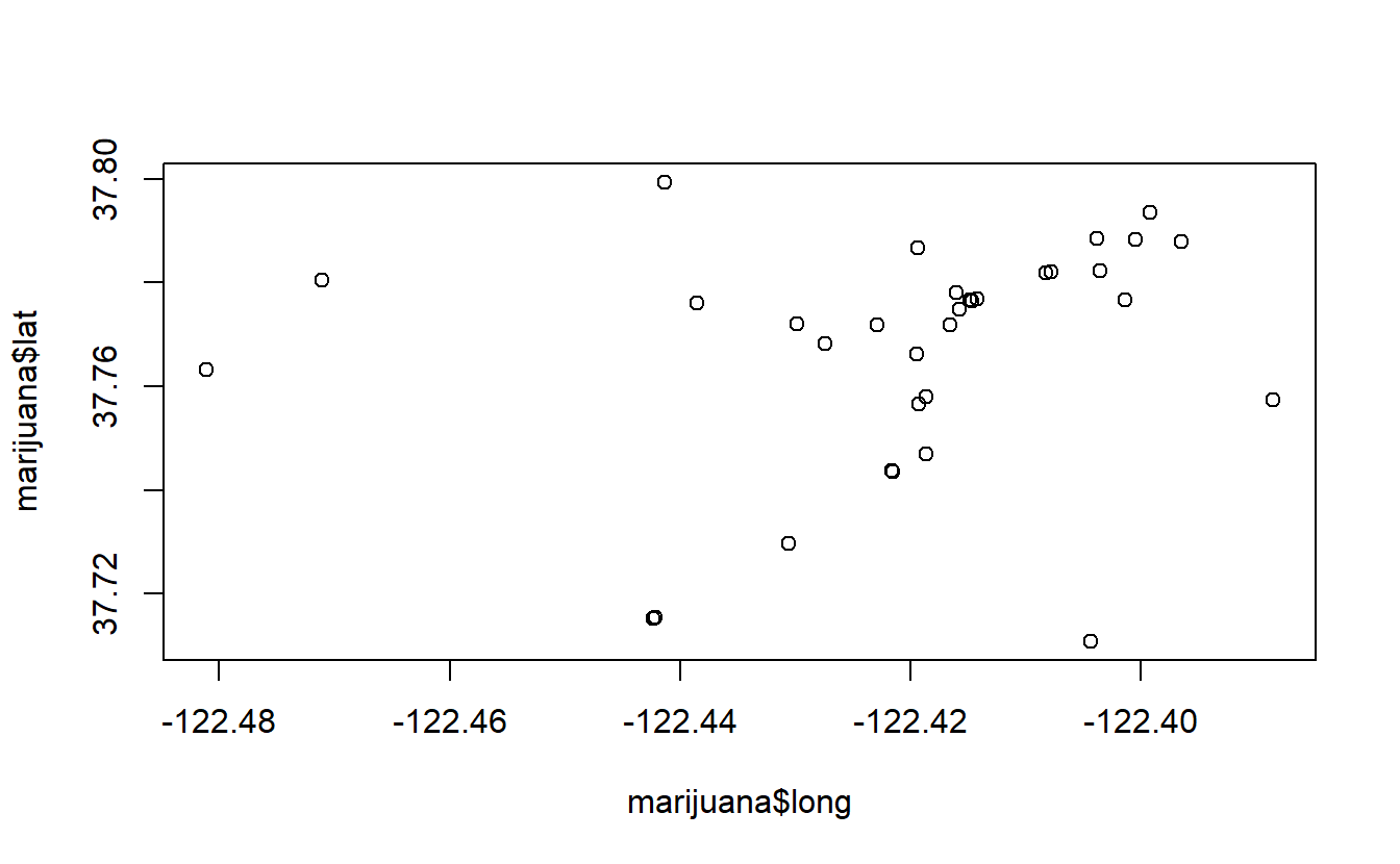
Most points are within a very narrow range so it appears that our geocoding worked properly.
We can look at all of the parameters for this function by running the code
help(geocode)or?geocode()to look at the functions Help page.↩︎